
About these pages
These pages measure a competition rule instead of judging it. The question is not whether the set system is fair, but how often, looking at a handful of arrows, it can tell which of two archers is shooting better, and how much that ability changes compared with the old cumulative score. The model is deliberately spare: an archer is the width of their group, and nothing else. No real archer's score enters the work.
Extended summary
The question
In 2009, individual recurve archery adopted the set system, which from 2010 onward became the format used across the major circuit. Matches were no longer decided by adding up the scores of every arrow: instead, they were divided into three-arrow sets, with two set points awarded for winning a set and victory going to the first archer to reach six. The federation stated that it wanted more open matches, less likely to be decided by a single disastrous arrow, and a format capable of rewarding consistency.
Ever since, the debate over whether the change was good or bad has largely remained a matter of opinion. But “fair” and “unfair” are words for a courtroom, not a target face: the relevant question for a measurement instrument is not whether it is fair, but how precise it is — that is, how often, from a limited number of arrows, it correctly identifies which of two archers shoots better.
Framed this way, the question has a numerical answer. This study calculates it, together with three consequences that have never been quantified: how often the set system produces the paradox of awarding the match to the archer with the lower raw score; whether it really favors the more consistent archer, as the federation intended; and, for comparison, how precise the qualification ranking used to assign seeds actually is.
Method
The model. Each arrow lands within a cloud of impacts described by a two-dimensional Gaussian distribution around the aiming point; the width of that cloud, σ, is the operational definition of skill used here. From the geometry of the 122 cm target face at 70 metres, the probability of each possible score can be derived, and from those probabilities the expected score over a 72-arrow round. The relationship is strictly monotonic and therefore invertible: for any given expected score, there is exactly one dispersion width that produces it.
The calculation is exact, not simulation-based. No probability is estimated by running virtual competitions: the total score over n arrows is obtained by convolution, while the set match is solved by backward induction over match states. None of the published figures carries sampling error, and repeating the calculation returns the same value to the final decimal place. The only approximations are deterministic — Gauss–Legendre quadrature for non-circular impact clouds, which in the circular case reproduces the exact formula to the eleventh decimal place.
There are no empirical data in the study, by design. No real archer’s score enters the analysis. The archers are synthetic and defined by their expected scores: the conclusions concern the competition format, not a population of athletes.
How the work was verified
Published equations — all twenty-four equations in the model are provided in the appendix, together with their domains, conventions, and limitations.
Reproducibility package — a script recalculates and checks, one by one, all 110 values printed in the paper; 35 tests verify structural properties; the computational environment is frozen and the code is released under an open licence.
Independent implementation — a second engine, written solely from the specification and sharing no code with the first, recalculates 34 quantities using different methods. The two agree within 1.4·10⁻⁵. Change any model parameter and the tests and verification checks fail: the test suite has teeth.
Results
1. The cost of the format is just over two matches per hundred. When the two aggregation methods are compared at the same number of arrows, cumulative scoring identifies the more precise archer slightly more often than the set system. The maximum gap is 2.32 percentage points: for the worst-case pair, cumulative scoring selects the correct winner 87 times out of 100, compared with 85 for the set system. Roughly two matches in every hundred change hands — one in forty-three.
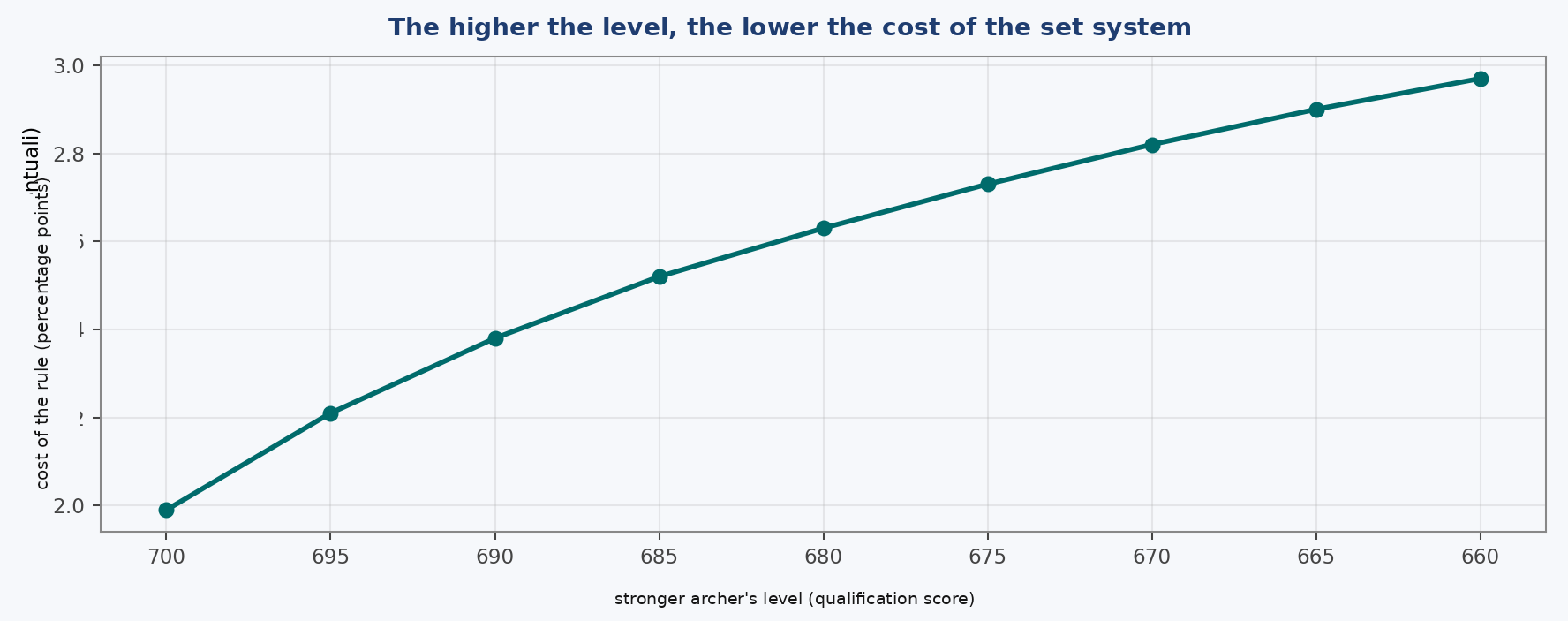
The cost depends on competitive level, and in a surprising direction: it is smaller at the top. It is 1.99 percentage points for a 700-level archer, 2.38 at 690, 2.82 at 670, and 2.97 at 660. The set format imposes a larger penalty farther from the elite, which means it is actually best suited to the level at which it is used.
2. The loss comes from the rule, not from the match being shorter. The most common defence — that the set system discriminates less well simply because fewer arrows are shot — is false, and four lines of arithmetic are enough to show why. Across five sets, ten set points are distributed. An archer who reaches six can have conceded at most four to the opponent, and at most four additional points remain available even if every unplayed set is completed. An archer who wins under the stop-at-six rule would therefore also win if the match were always played to full distance, for every pair of archers and every possible match realization. The calculation confirms this: the two match versions produce identical probabilities, with exactly zero difference.
The entire gap therefore comes from the aggregation rule itself. The countercheck is that making the match longer does not help: three sets versus nine arrows produces a 1.84-percentage-point gap, five versus fifteen produces 2.32, and seven versus twenty-one produces 2.38. Every additional set creates another boundary at which margin information is discarded — because within a set, winning by one point counts exactly the same as winning by ten, and that difference does not carry across the boundary. For the reference pair, a won set is won by an average of 1.76 points, and by two or more points in more than half of all cases.
3. The paradox is common, but not where one might expect. A lower raw-score winner occurs in 7.1% of matches between essentially equal elite archers — about one match in fourteen — and becomes more frequent at lower levels: 9.2% at 670 and above 10% at 650. Yet the rate is highest precisely where the cost is zero: between identical archers, reversals are very frequent, but none is an error because there is no more precise archer to betray. As the skill gap widens, reversals become rarer, but each one increasingly represents a genuine misclassification. The format looks most scandalous where it makes the fewest mistakes.
4. The result that reverses the rule-makers’ stated intention
The set system was adopted in part to reward consistency. Compare a consistent archer with an inconsistent one who produces the same mean score, with the latter having one arrow in twenty drawn from a cloud three times wider. The consistent archer wins 48.5% of matches under cumulative scoring but only 45.4% under the set system.
The set format protects the archer who makes an extreme error because the catastrophic arrow is contained within the set in which it occurs: the archer loses that set rather than compromising the total score. The weakness becomes a shield, and a shield necessarily protects someone. This is the opposite of what the rule change was intended to achieve.
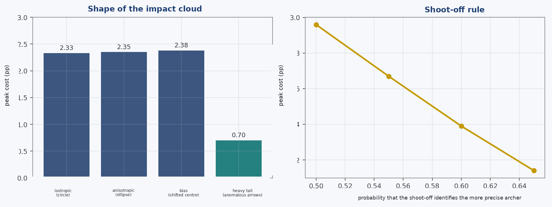
5. The conclusion survives changes in assumptions. Distorting the impact cloud changes almost nothing as long as the model is recalibrated to the same expected score: circular, 2.32 percentage points; vertically elliptical, 2.34; group shifted by three centimetres, 2.36. The only deformation that matters materially is a heavy tail, which cuts the cost to less than one third (0.68) — consistent with the result on consistency, because it is the same mechanism viewed from another angle. A more centrally concentrated cloud, by contrast, increases the cost: raising the stronger archer’s X rate from 22% to 30% moves the gap from 2.32 to 3.13 percentage points.
Across 64-archer fields constructed from four different profiles, the top seed’s probability of winning gold is always higher under cumulative scoring, and the difference remains between 3.3 and 4.3 percentage points:
Across four 64-archer fields, the top seed’s probability of winning gold is always higher under cumulative scoring: 30.9% versus 34.5% when many rivals are clustered near the top, and 58.4% versus 62.7% when the leading archer is clearly separated from the field. The difference stays between 3.3 and 4.3 percentage points in all four cases, whereas the first and second field profiles differ by twenty-seven points: field composition matters roughly ten times more than the scoring rule, while the format effect is small and remarkably stable. The four percentage points lost by the favorite do not disappear — every tournament still awards a gold medal. In the linear field, +1.9 points go to seeds 2–8 and +2.3 to seeds 9–32: the set system transfers winning probability from the favorite to outsiders, the same consistency mechanism viewed at tournament scale.
6. Qualification noise is larger than the effect being studied. Two identical archers each shooting a 72-arrow round finish an average of five points apart purely by chance (standard deviation of the difference: 6.30). To conclude with 95% confidence that one is genuinely better than the other requires a gap of a little over ten points. A five-point gap corresponds to 79% confidence, eight points to 90%, and twelve points to 97%.
7. Detecting a real improvement requires far more competitions than people usually examine. The variability of a single competition cannot be removed, but it can be diluted by averaging: it falls with the square root of the number of rounds, so four competitions halve it and nine reduce it to one third. This determines how many competitions are needed before and after a technical change. For an archer around 650: twenty-nine competitions per period to detect a three-point improvement, eleven for five points, five for eight, and three for ten. At 690, the same three-point improvement requires thirteen competitions because total-score variability is lower. Gaining three points over a season is excellent technical progress; demonstrating it statistically requires two seasons of measurements.
The implication is that a technical change should not be judged by short-term score: the score simply lacks the resolution to detect it. It should instead be judged through what can be observed directly — movement repeatability, group shape, video — while score, averaged over a sufficiently long block, is left to confirm the change months later.
These are the most useful findings for coaches, and they also put everything else into perspective: considerable attention is devoted to an arithmetic rule that changes roughly two matches in a hundred, while the qualification ranking used to assign seeds cannot reliably order most closely matched pairs.
What the study does not claim
The model assumes independent arrows, constant dispersion within a round, no dependence between the two archers, and no strategic or pressure effects. Every assumption is listed in the appendix together with the direction in which the result would be expected to move if that assumption were violated.
Most importantly, none of this says whether the set system is the “right” format. Competition formats are also chosen for duration, spectacle, and perceived fairness, none of which enters a probability calculation. This study measures one property only: the ability to identify the more precise archer. What should be done with that information is a decision — and numbers do not make decisions.
The day archery changed its arithmetic
In 2010, recurve archery changed a single rule — and not one of the visible ones. The distance remained seventy metres, the target remained a 122-centimetre disc, and neither bows nor arrows changed. What changed was the arithmetic used to decide which of two opponents advanced and which went home; in a knock-out sport, that is ultimately the only outcome that matters. The transition was not as clean-cut as is sometimes remembered: the set system entered individual recurve in 2009 and became the format across the entire major circuit the following year. Even then it was not yet uniform: elimination rounds used six-arrow sets, while the three-arrow sets used in every match today applied only from the quarter-finals onward.
Until then, matches had been decided by adding scores: the archers shot a fixed number of arrows and the higher total won. From that point onward, matches were decided in sets: three arrows at a time, the set going to whoever scored higher over those three, and the match to whoever first won the required number of sets. These are two different ways of reading exactly the same arrows. And in the very same contest, they can produce different winners.
The international federation did not hide its reasons. Under the old system, a match could be essentially lost after a single end because of one poor shot: a disastrous arrow could make the cumulative deficit impossible to recover. The set format was adopted to prevent that, to reward consistency, and to keep matches alive until the end.
Ever since, people have argued over whether the change was good or bad, and the debate has largely remained a matter of opinion: some regard the set system as fairer, while others accuse it of gifting victories. But fair and unfair are courtroom words, not target-face words. A competition format has no morals; it does not reward virtue or punish fault. It does something more modest and, in the end, more interesting: it measures the performance of two people and converts that measurement into a verdict.
And the question to ask of a measurement instrument is not whether it is fair, but how precise it is — how often, from a limited handful of arrows, it actually identifies which of two archers shoots better. Unlike the question of whether something feels unjust, this question has an answer. And the answer is a number that can be calculated without shooting a single arrow.
What happens in an Olympic competition: qualification, seeding, bracket
Start with the basics, because the structure of the competition is precisely why the question matters.
An Olympic individual recurve event unfolds in two phases. The first is the qualification round, which does not eliminate anyone: every competitor shoots seventy-two arrows at seventy metres on a 122-centimetre target face. The theoretical maximum is 720 points. That score does not award a medal. It orders the archers from first to last and assigns each of them a seed.
The target face consists of ten concentric scoring rings, all the same width: 6.1 centimetres. An arrow landing within the innermost circle, whose radius is 6.1 cm, scores ten; the next ring scores nine; and so on down to one in the outermost ring, whose outer boundary lies sixty-one centimetres from the centre. Outside that boundary, the score is zero. Inside the ten there is an even smaller circle, 3.05 cm in radius, called the X ring. It is still worth ten points and is used only to break ties.
To appreciate the scale of the task, it helps to translate it into something familiar. At seventy metres, the entire 122-centimetre target face occupies roughly the same visual angle as a two-euro coin held about a metre and a half away. The ten ring, 12.2 centimetres in diameter, corresponds to that same coin viewed from roughly fifteen metres away. A truly elite score, around 710 out of 720, means putting more than eight arrows out of ten inside that coin-sized visual area, seventy-two times in succession.
The second phase is the elimination bracket: thirty-two matches in the first round, sixteen in the second, then eight, four, two, and the final. Winning gold requires six consecutive victories. Each match is an extremely short measurement — at most fifteen arrows — and everything depends on it.
Two kinds of arithmetic: the set system and cumulative scoring
Cumulative scoring is the intuitive way to count: each archer shoots fifteen arrows, the scores are added, and the higher total wins. If the totals are exactly equal, each archer shoots one additional arrow and the arrow closest to the centre wins: the tie-break, or shoot-off. This is still the system used today for compound matches.
The set system differs in only one respect, but that one difference changes everything. The match is divided into three-arrow sets. The archer with the higher score in a set receives two set points; if the set is tied, each receives one. The first archer to reach six set points wins the match. At 5–5, the match goes to a shoot-off: one arrow each, closest to the centre. Because set points accumulate and are never taken away, the match ends the instant one archer reaches six. It can therefore finish in three, four, or five sets — nine, twelve, or fifteen arrows.
The difference sounds technical, but it has a consequence worth seeing with real numbers. Consider a set-system match that goes the full five sets.
| Set | Archer A | Archer B | set points |
|---|---|---|---|
| 1st | 30 | 26 | 2 – 0 (A) |
| 2nd | 27 | 28 | 2 – 2 (B) |
| 3rd | 28 | 29 | 2 – 4 (B) |
| 4th | 30 | 25 | 4 – 4 (A) |
| 5th | 27 | 28 | 4 – 6 (B) |
| Total | 142 | 136 | B wins |
A put six more points on the target than the opponent and still lost the match 4–6. This is neither an anomaly nor a calculation error: it is the system working exactly as designed. The set system does not count total points; it counts won moments. Winning a set by four points is worth exactly the same as winning it by one, and any margin accumulated inside a set already won is useless thereafter. A dominated where the extra margin did not matter and narrowly lost where it did.
This is the very property for which the format was chosen, viewed from the other side. If one disastrous arrow costs you only the set in which it occurs, the damage is contained. But by symmetry, surplus points cannot escape the set in which they were scored either. Robustness and paradox are two sides of the same coin. Later we will quantify how often this happens.
What does “better” mean?
To measure how often a format identifies the better archer, we first have to define what “better” means. And that definition must be fixed before looking at the results, not after them: this elementary precaution supports everything that follows. If we defined the better archer as the one who won, every format would be perfect by construction and there would be nothing left to measure.
Here, skill means one thing only, fixed in advance: raw shooting precision, or how tightly the archer groups arrows on the target. It is deliberately a stripped-down definition. It is not complete competitive ability: it excludes composure under pressure, wind reading, tactical management of sets, and nerves on the shoot-off arrow. We do not claim that precision is everything. It is simply the quantity we ask each format to recover, and every number that follows measures how much information about that quantity each rule preserves.
The group and its spread
Fortunately, an arrow group can be described by a single number. Imagine decomposing every error into two independent components: how far the arrow lands to the right or left of centre, and how far above or below it. If each component follows a Gaussian bell curve — the standard assumption for measurement errors ranging from a reading on a scale to a star’s position measured through a telescope — and both have the same spread, then the arrow’s radial distance from the centre, which is the only quantity that determines score, follows what mathematicians call a Rayleigh distribution.
The Rayleigh distribution has one parameter, denoted by the Greek letter sigma and measured in centimetres. Sigma is the characteristic spread of the group: a small sigma means a tight group and an extremely precise archer; a large sigma means a wider group. That single number is the archer’s signature, and it contains everything the model knows about that archer.
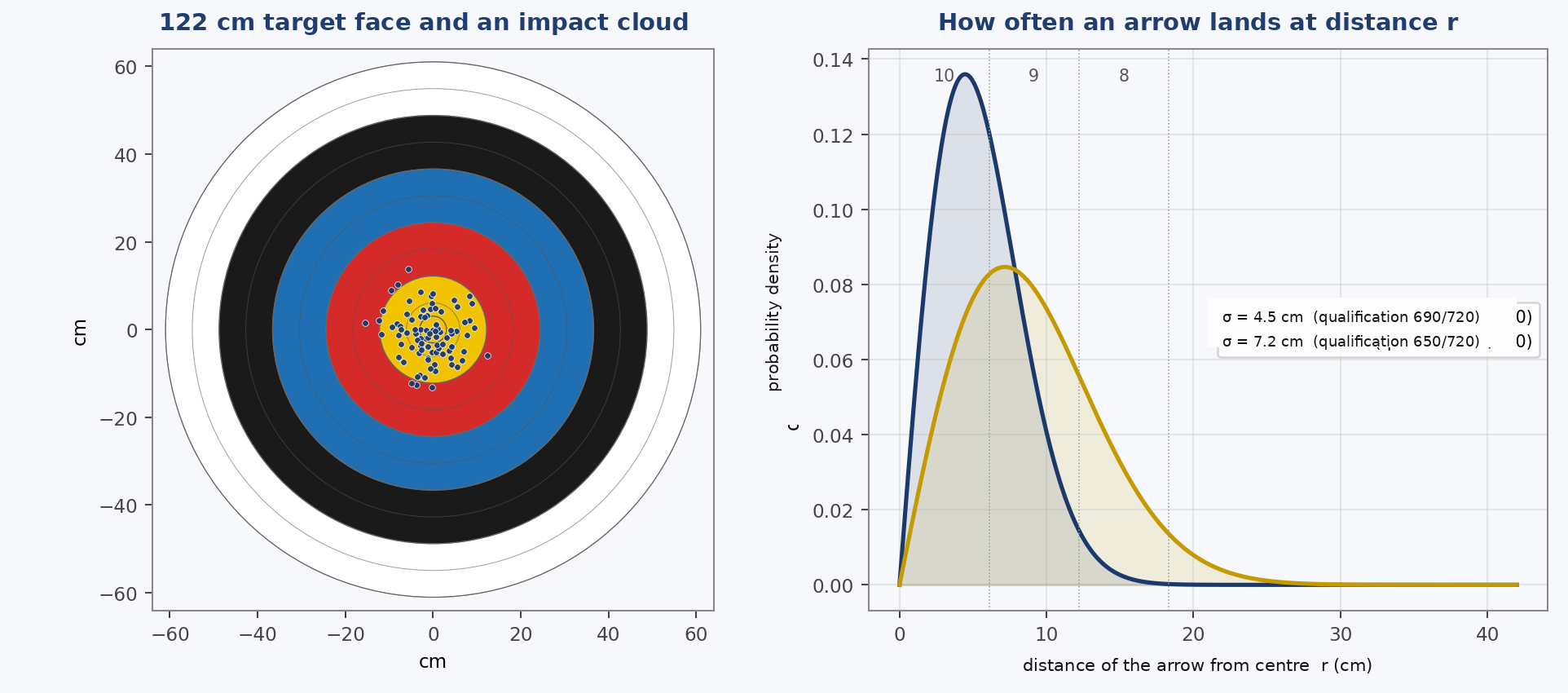
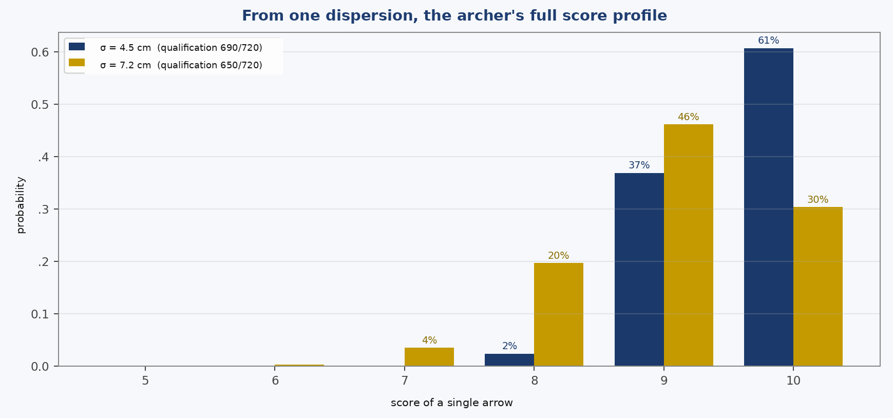
Because the scoring rings are concentric annuli with known widths, the probability of scoring exactly ten, nine, eight, and so on is simply the probability of landing inside the outer boundary of that ring minus the probability of landing inside its inner boundary. Two subtractions yield the probability of every possible score.

A single spread therefore determines the archer’s entire probability profile: the exact probability of scoring ten, nine, eight, and so on with every shot. An archer with an expected 72-arrow score of 690 has a group with a spread of about 4.5 centimetres and puts roughly six arrows out of ten into the ten ring; a 650-level archer has a group just over seven centimetres wide and hits the ten only about three times in ten. A physical property — how tightly the arrows are grouped — has become a precise list of probabilities.
From a score to a spread
The relationship also works in reverse, which is what makes the model usable. Because the probability profile depends on sigma, so does the mean score per arrow and therefore the expected total over seventy-two arrows. The relationship is monotonic: the tighter the group, the higher the total, without exception. It can therefore be inverted: given a mean score, we find the unique spread that produces it. Inferring that spread from an observed score, however, is a different matter, and later we will see the price of doing so: a single 72-arrow round leaves the spread uncertain by more than a centimetre.
The result is a map that translates ranking-round points into centimetres of spread, and it has a counterintuitive property worth examining. Across the entire range that matters, from 630 to 700 points, the relationship is almost perfectly linear, with a slope just under seven hundredths of a centimetre per point. In more practical terms, a single qualification point corresponds to about seven tenths of a millimetre of spread. Eight points, which look like a chasm on a results sheet, correspond to barely five and a half millimetres — essentially the same conversion at both ends of the range.
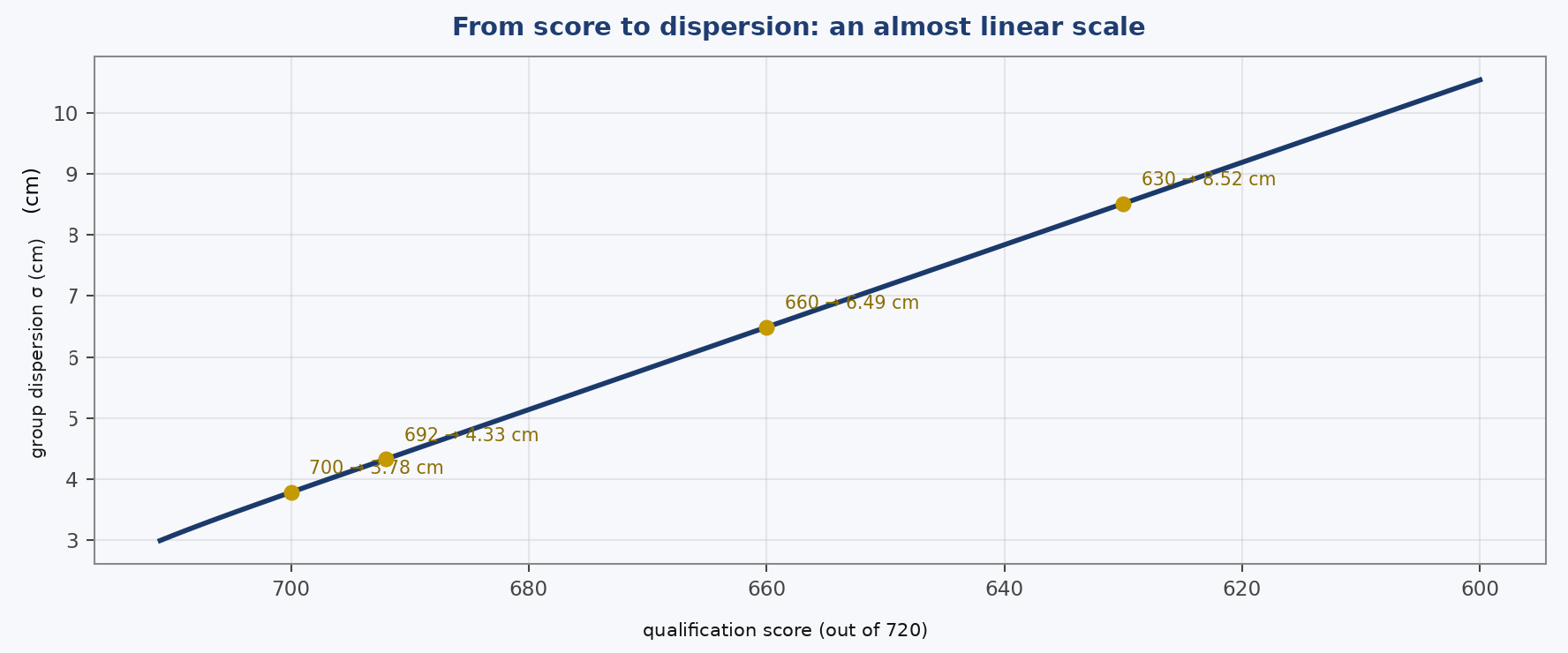
The curve steepens only at the extreme upper end, above 700 points, where further gains require the group to collapse towards zero. Everywhere else, the conversion is remarkably uniform, and that is the important point: fewer than five centimetres of spread separate an elite 700 from a 630 at the lower end of the field, while two archers separated by a single ranking point differ by less than a millimetre. On the target, there is almost nothing between the champion and the near-champion. Keep that in mind, because it explains much of what follows.
How to calculate a competition that was never shot
We now have one number for each archer; what we still need is the machinery that converts those numbers into winning probabilities. That machinery is really several distinct components, each with a precise task, and they are best taken one at a time.
The first component adds arrows together and is called convolution. The name sounds intimidating; the idea is elementary-school arithmetic. If I know the probability of every score on a single arrow, I can derive the probability of a two-arrow total by counting every way of reaching it — nineteen can be ten plus nine or nine plus ten; eighteen can be obtained in three different ways — and weighting each route by its probability. The operation combines two arrows at a time and is then applied again to the result: the distribution for two arrows combined with that for one arrow gives the distribution for three — one set — and continuing in the same way eventually gives fifteen arrows: a cumulative-score match. Comparing the two archers’ total-score distributions yields the exact probability that the more precise archer wins.
The second component handles the set system, which is not a simple sum but a process with memory: three arrows, someone wins the set and leads 2–0; three more, perhaps the match reaches 2–2; and the contest ends the instant one archer reaches six set points, not one arrow later. It can be calculated like a board game. Draw a grid of states — each square is a possible set-point score such as 0–0, 2–0, 2–2, 4–2 — and from each state we already know the probabilities of moving to the next one because those are just the set probabilities calculated above. Summing the probability of every path that ends in A winning gives A’s exact match-win probability. Mathematicians call this an absorbing Markov chain because some states — those in which one archer reaches six set points — cannot be left: once a player enters one of them, the match is over.
The third component handles shoot-offs, and it has a surprisingly clean closed-form expression. The rule needs stating precisely: victory goes first to the higher-scoring arrow, with closeness to the centre used only if the scores are tied. But because the scoring rings are concentric, those two formulations always identify the same winner: the arrow closer to the centre can never have a lower score than the other. Treating the shoot-off as a comparison of radial distances, the probability that A wins depends only on the ratio of the two spreads: it is sigma B squared divided by the sum of the two squared sigmas. If the groups are identical, the probability is exactly one half, as it must be. Between a 690-level archer and a 665-level archer it is a little over 65%, meaning that the more precise archer is favoured but the weaker archer still has a very substantial chance. The same shoot-off rule is applied to both formats, because granting one format a tie-break while denying it to the other would bias the comparison.
One final component is needed for a specific question: how often does the set-point winner finish with fewer raw points than the opponent? To answer that, it is not enough to calculate who wins and then inspect the totals afterwards, because the two quantities have to be tracked jointly, set by set. The engine therefore carries a second counter alongside the set-point state: the accumulated raw-score difference. In each set, the sign of the difference between the two three-arrow totals determines who wins the set, while its magnitude updates the cumulative margin. At the end, the probabilities of all terminal states in which the match winner has the lower raw total are summed.
One final clarification: simulation is never used to generate a published result. The competition is not run ten thousand times in the hope that the average will be close to the truth. Every probability is calculated in full, to the final numerical digit. A simulation returns an answer blurred by randomness — run it again and it changes slightly — whereas exact calculation returns the answer without that noise. When we later read that a particular difference is 2.32 percentage points, that value carries no sampling error: anyone repeating the calculation tomorrow, or on another machine, will obtain the same value to the last computed decimal place. Random sampling appears only once in these pages, and for a different purpose: as an external validation of a numerical integration, never as the source of a published figure. Numbers in the text are rounded to two decimal places, as is customary; the accompanying code retains their full precision.
The calculation engine
The calculations were not done by hand. Behind them is a purpose-built computational engine: it takes target geometry, the spreads of two archers, and the rules of a competition format, and returns the exact probabilities of every outcome. It produced every table and figure in this study, and I shall explain how it was built, because readers are entitled to know what performed the calculations and what backs them up.
The engine was written with the assistance of an artificial-intelligence system from a specification that fixes the mathematics module by module: target-face geometry, the dispersion model, the arrow generator, inversion from score to spread, match formats, and trajectory ballistics. This needs saying plainly. It is even more important to explain what that does — and, especially, what it does not — mean.
An AI system wrote code; no AI system guessed the results. That distinction is the whole point. The code implements closed-form mathematics — the Rayleigh distribution, convolution of score totals, backward induction over set-point states — that is exactly what one would calculate by hand given unlimited patience. There is no learning, no training on past competition results, and no prediction model. There is arithmetic, executed quickly and identically every time: given the same inputs, the engine returns the same outputs because there is nothing to infer. Every step is the evaluation of a defined function.
This is not a semantic distinction, because it changes what can be audited. A system that learned from past competitions and guessed the winner would be a black box: one could only trust it or not. An engine that evaluates a stated formula can be checked line by line: read the specification, repeat the calculation, verify the number.
That verification was performed at three levels. The first is the most basic and the most necessary: more than one hundred automated tests cover the engine as a whole, each linked to a criterion stated in the specification, and all must pass before the engine is considered usable. More than twenty of those tests are included in the package distributed with this study and specifically cover the modules and calculations used in these pages. Anyone downloading the package can run them with a single command and watch them pass, together with a script that recalculates every number printed in the study and compares it with the published value.
The second level concerns formulas for which no analytical solution exists. Where a closed form is available, the engine uses it because it is exact and immediate. Where none exists — elliptical groups, shifted centres, mixtures containing anomalous arrows — numerical integration is used instead. That raises a question that is rarely asked: how approximate is the approximation?
The obvious answer would be to compare numerical integration with the exact formula in the isotropic case, the only case in which such a formula exists, and indeed the two agree to the eleventh decimal place. But that comparison alone is not enough, and it is worth understanding why. In a circular group, density is the same in every direction, so the angular component of the calculation simplifies away. An integrator that made an error precisely in that component — the most natural place for an error, and the part that matters as soon as the group becomes elliptical — could pass the isotropic test perfectly while still being wrong on every deformed-group case that matters here.
The required validation is therefore different, and it must be performed on the deformed shapes themselves. A very large sample is drawn directly from the true distribution — twenty million shots — and its resulting mean score is compared with the value predicted by numerical integration. For a 1.5:1 ellipse, an intentionally extreme 3:1 ellipse, and a group shifted three centimetres from centre, the discrepancy remains only a few thousandths of a point per arrow, the same scale observed in the circular case. In other words, the angular dependence is handled correctly: not because we assume it is, but because it was tested precisely where it could have failed.
The third level matters more, for a study like this, than all the others combined. Every number in these pages was recalculated by a second implementation, written independently from the same mathematical specification: different code, different programming choices, and not a single line shared with the first implementation. The two engines were compared across thirty-four quantities, from zone probabilities to gold-medal probabilities across a bracket, and they agree to within one hundred-thousandth in relative terms — roughly five significant digits — with the residual attributable to numerical quadrature error rather than disagreement over the result. This is among the strongest available safeguards against implementation errors, because the probability that the same coding error appears identically in two independent implementations is far smaller than the probability that it appears in one. What this means is easy to overlook, and it is the strongest guarantee these pages possess. These are not two runs of the same program, which would of course return the same result; they are two independent translations of the same mathematics, produced at different times and using different data structures. If they agree to five digits over thirty-four distinct quantities, either both are correct or both made the same mistake independently. This does not, of course, protect against an error in the specification itself: if the written formula is wrong, two faithful implementations will reproduce the same wrong formula. That is why the equations themselves are published, rather than only the numbers derived from them.
None of these checks proves that the model describes reality well. That is a separate question, and the relevant limitations are listed later. What the checks establish is something more modest but still necessary: the reported numbers are genuinely what the stated equations produce. A validated engine can be wrong because the model is wrong; it is not wrong because the arithmetic was implemented incorrectly.
The verdict: what does the set system cost?
Now we can run the engine. Fix a strong archer — an Olympic-elite level of 692 out of 720, corresponding to a group about 4.3 centimetres wide — and gradually widen the opponent’s group, starting from exact equality and moving downward in performance. At every gap, ask both scoring systems the same question: with what probability does each one crown the more precise archer?
At the extremes, both behave as they should. At exact equality there is no more precise archer to identify, so each splits matches fifty-fifty; with a very large skill gap, each is effectively infallible. Everything happens in between. In that middle region, cumulative scoring is the better judge: it more often identifies the archer with the tighter group — in statistical terms, it is the better discriminator — although, as we are about to see, its advantage is much smaller than archery debates tend to suggest.
Fix the unit of measurement now, because it will recur throughout the study. One percentage point means one match per hundred: if one rule identifies the better archer 80 times out of 100 and the other 78 times, the difference is two percentage points — two matches per hundred, not two per ten, as a quick glance might suggest. With that unit in mind, the result is that the set system’s maximum disadvantage is 2.32 percentage points, reached at an intermediate gap: an opponent around 675 against the stronger archer’s 692, just under a quarter of a point difference per arrow.
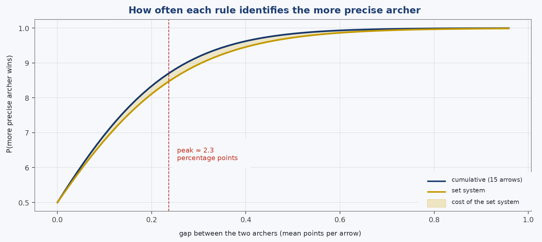
The shape of that band reveals something important and dispels a common misconception. The disadvantage is not largest between almost equal archers, as one might expect, but in the middle. Once stated, the reason is obvious. When two archers are nearly identical, no competition format in the world can do much better than a coin toss: the contest truly is close to fifty-fifty, and resolving it randomly is not a measurement failure but an honest reflection of the uncertainty. When one archer is clearly stronger, every reasonable rule identifies that difference easily. Only in the intermediate range does the choice of format have information to lose.
This leads to the first lesson, perhaps the most important for athletes and coaches: a single upset between similarly matched archers proves nothing. It does not show that the format is unfair, that the loser was actually stronger, or that the winner somehow stole the match. Between near-equals, the coin is genuinely in the air and can land either way. Treating one result as a definitive judgement of their relative ability is a measurement error, not a sporting insight.
The cost depends on performance level: where the set system penalises most
There is a detail that is usually missed, and it matters because it prevents us from treating 2.32 as a universal constant. The cost of the set system depends on the absolute performance level of the two opponents, not only on the gap between them. And the direction is surprising: the stronger the archers are, the smaller the cost of the format.
| level of the stronger archer | peak cost |
|---|---|
| 700 points | 1.99 pp |
| 692 points | 2.32 pp |
| 680 points | 2.63 pp |
| 670 points | 2.82 pp |
| 660 points | 2.97 pp |
Between a world-class match and a strong national-level match, the format cost rises from just under two percentage points to almost three. The reason is that at the very highest level, most arrows land in the ten, set scores become highly similar, and the difference between the two arithmetic systems narrows. Lower down, where set scores vary more, the aggregation rule matters more. This has a practical implication: the set system’s disadvantage is smallest precisely where the format is used — at the top of the sport.
The culprit is the set rule, not the short match length
At this point, one explanation comes naturally. The set system is designed to end early: the moment one archer reaches six set points, the match is over, and that can happen after nine or twelve arrows rather than the full fifteen of cumulative scoring. Anyone who measures anything knows the general rule: a shorter measurement is a noisier measurement. If the set system decides matches from fewer arrows, the argument goes, it is only natural that it should discriminate a little less well, and the culprit would be the short sample rather than the way the points are counted.
It is a reasonable explanation, and it is wrong. The claim can be dismantled with a test anyone can reproduce: take the same set match used by the engine and force it to play all five sets to completion, even after one archer has already reached six set points, then award the match to whoever has more set points at the end. If the shorter match carried a cost, the full-length version should discriminate better. It does not. The two versions yield exactly the same win probability — not approximately the same, but identical to the last numerical digit the computer can represent.
Once seen, the reason is elementary, although compressing it into one sentence can make it seem as if a step has been skipped. Across five sets, exactly ten set points are distributed, two per set regardless of the outcome: two to the set winner, or one each if the set is tied. That total is fixed, and nothing else is needed.
It is not true that someone always reaches six. In roughly one match out of five between equally matched archers, all five sets end with the score tied at 5–5: all fifteen arrows have already been shot, the match proceeds to a shoot-off, and the short and forced-full-length versions are identical. The issue arises only when one archer reaches six set points, which can happen after three, four, or five sets. In every case the same question applies: could the opponent catch up by playing the remaining sets?
If the match ends after three sets, the winner must have won all three and the opponent is on zero; two sets remain, worth at most four points. If it ends after four, the winner can have conceded at most two points, because eight set points have been distributed and six belong to the winner; one set remains, worth at most another two. If it ends after five, the loser can have at most four and there is nothing left to play. Three different paths, one conclusion: the losing archer can never get beyond four set points against six or more for the winner, leaving a margin of at least two.
The arrows the set system does not require are exactly the arrows that could not have changed the verdict. Stopping early is not a saving purchased at the cost of precision. It is free.
That removes the excuse, and under this model the set system’s small disadvantage must be attributed entirely to the aggregation rule. Look then at what the rule actually does, because the mechanism fits in one sentence: within a set, winning by one point is worth exactly the same as winning by ten. The margin is reset at the set boundary and does not carry forward. In the region where format matters most, a won set is won by an average of 1.76 points, and in half of all cases by two points or more. That is the information cumulative scoring retains and the set system discards, set after set.
The most elegant test of this interpretation is to change the number of sets and observe what happens. If short match length were the cause, lengthening the match should reduce the disadvantage because more arrows are being observed. The opposite happens, and the pattern is more informative than the conclusion itself.
Start with the limiting case. With only one set, the gap between the two formats is exactly zero: the archer with more set points is necessarily also the archer with more raw points, because there is no internal boundary across which information can be lost. The cost appears from the second set onward, at the exact moment the first wall is introduced. It then grows: three sets compared with nine-arrow cumulative scoring produce a 1.84-percentage-point gap; the regulation five sets against fifteen arrows produce 2.32; seven sets against twenty-one arrows produce 2.38.
Then the gap stops growing. At nine sets it has already fallen back to 2.27, at thirteen to 1.85, and by twenty-one sets — sixty-three arrows — it is just over one percentage point. Two forces are acting in opposite directions. Every extra set adds another boundary at which score margin is discarded, but every extra set also adds three arrows, and with enough arrows both formats become almost infallible. At twenty-one sets, cumulative scoring identifies the more precise archer in 98.8% of matches and the set format in 97.8%; there is no room above 100% for a large difference. The maximum cost therefore occurs where the two effects balance, around six sets, and the regulation five-set match stops just short of that peak.
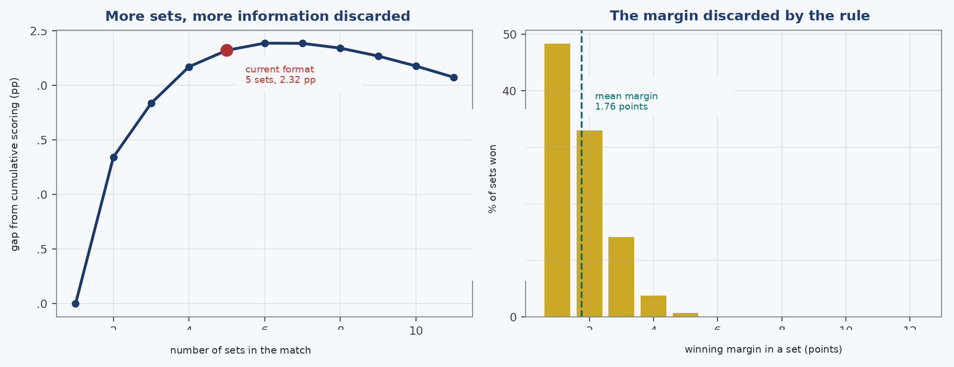
The verdict is therefore the opposite of common intuition, but also the opposite of the more sophisticated alternative explanation. The problem is not that the match is short. The set rule itself — the feature everyone points to — is what costs roughly 2.3 percentage points. What differs from the popular accusation is not the culprit, but the magnitude.
Here is what those 2.3 points mean, once and for all. At the worst point, with a 692-level archer against a 675-level opponent, cumulative scoring identifies the more precise archer in 87 matches out of 100 and the set system in 85. Roughly two matches in a hundred change hands: one in forty-three, twenty-three in a thousand. An archer who contested one hundred matches of that type over a career would lose about two matches that the other arithmetic would have awarded to them, and win about two that the other arithmetic would have lost.
And this occurs only across an intermediate range of skill gaps. Between equal archers the cost is exactly zero because there is no more precise competitor to identify. At a two-point gap the cost is about half a percentage point; at five points, a little over one; it rises to a maximum around seventeen points and then falls again. At a thirty-five-point gap it is just over one percentage point, and at forty-five it is about 0.6. Calling the set system a “lottery” implies effects measured in tens of percentage points. The calculation finds a little over two, and only where the archers are close enough for the question to matter but far enough apart for a correct answer to exist.
The paradox of winning with fewer points
Return to the example match from the opening pages, in which A scored 142 against B’s 136 and still lost 4–6. That was not a contrived curiosity. It is an outcome with a precise frequency, and we can now quantify it.
The quantity is the paradox rate: the probability that the set-point winner finishes with the lower raw total. It can be measured in two legitimate ways. The first compares totals over the arrows actually shot — nine, twelve, or fifteen, depending on when the match ended — which is what a spectator would see on the scoreboard. The second compares totals over fifteen arrows, as if the match had always been played to full length, and asks the counterfactual question: who would have won if all five sets had been completed? This is not the old recurve cumulative format, which used twelve arrows; it is fifteen-arrow cumulative scoring, the format now used in compound, chosen here because it compares the two arithmetic systems with the same maximum number of arrows.
Between two essentially equal elite archers, the paradox rate is 7.1% when totals are compared over the arrows actually shot and 7.6% when the match is hypothetically completed to fifteen arrows: roughly one match in fourteen. The frequency rises at lower performance levels. Between equal 670-level archers it is already 9.2%, and at 650 it exceeds 10%, or about one match in ten. The reason lies in the margins of individual sets, which vary much more at lower levels: between elite archers a set is typically won or lost by only a little over one point, whereas in the middle of the performance range the margin is roughly twice as large. More variable set margins make the paradox-generating configuration more likely — one heavy set loss combined with several narrow set wins. By contrast, at the point where the format has its largest discriminative cost — a 692-level archer against a 675-level opponent — the paradox rate falls to 4.7%, or about one match in twenty-one, and to 5.2% under the fifteen-arrow counterfactual comparison.
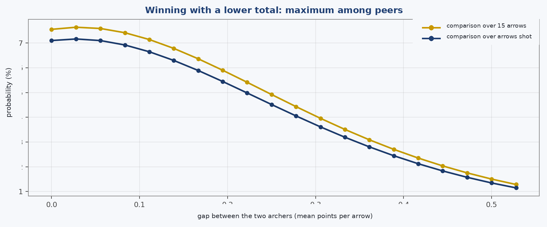
There is a regularity here that needs to be understood because it corrects the instinctive sense of outrage. The paradox is not most frequent where the format is least efficient. As we saw, discriminative cost peaks at intermediate gaps; the paradox, by contrast, becomes more frequent as the two archers become more similar, and reaches its maximum near equality, precisely where discriminative cost is zero. Between identical archers, reversals are common — about one in fourteen — and none is an error because there is no more precise archer to betray. As the gap widens, reversals become rarer: about one in twenty-one at a seventeen-point gap, one in thirty-three at twenty-five points, and one in sixty-nine at thirty-five. The format looks most scandalous where it makes the fewest errors, and makes more consequential errors after the apparent scandal has largely disappeared.
The reason is simple and defuses much of the controversy. For the match winner to have the lower raw total, the two totals must be close; and totals are close when the two archers are close. The paradox is therefore most frequent exactly where neither competitor had a much stronger claim to victory than the other. When one archer is clearly more precise, that archer’s total is almost always higher as well, and the paradox disappears.
Evidence that the result does not depend on the shape of the group
A sceptic could raise a fair objection here: the entire calculation rests on a perfectly circular group centred on the aiming point, whereas real groups are often somewhat oval, more elliptical, sometimes shifted to one side, and occasionally contain an arrow that is completely out of place. Each objection can be tested directly by deliberately deforming the model and repeating the calculation at the same mean score.
| group model | peak cost (percentage points) |
|---|---|
| isotropic — centred circle | 2.32 pp |
| anisotropic 1.5:1 — vertical ellipse | 2.34 pp |
| 3 cm bias — shifted centre | 2.36 pp |
| heavy tail — 5% anomalous arrows | 0.68 pp |
A word about how such a test must be run, because this is an easy place to make a serious mistake. and the lesson extends well beyond this study. It is not enough to deform the group; it must also be recalibrated, meaning narrowed or widened until the archer once again has exactly the same mean score as before. If this is not done, stretching a group into an ellipse does not merely change its shape, it also makes the archer worse. A 692-level circular archer stretched to a 1.5:1 ellipse without recalibration is actually worth about 675 points. The calculation would then be measuring a performance-level difference while mistakenly attributing it to shape.
This distinction is not pedantic because it changes the conclusion. Without recalibration, shape would appear to move the format cost by about four tenths of a percentage point; with recalibration, it moves it by about two hundredths. That is the kind of mistake that turns invariance into an apparent effect. The principle is worth remembering whenever two conditions are compared: hold constant the underlying quality of the archer and vary only the feature being studied, otherwise the analysis measures a hidden change in performance instead of the intended variable.
The first three rows tell the same story in three different ways. Compressing the group into an ellipse whose vertical axis is 1.5 times the horizontal — the kind of deformation associated with a systematic draw-length or release error — moves the cost by only a few hundredths of a percentage point. Shifting the entire group three centimetres off centre, as might happen with a poorly adjusted sight or a constant uncompensated wind, changes it by less than four hundredths. With effects this small, it is reasonable to suspect numerical noise rather than a real phenomenon, so that possibility must be excluded. The deformed cases have no closed-form solution and require numerical integration; but when that integration is tested on the isotropic case, where the exact formula is available, it reproduces the answer to the eleventh decimal place. The difference between the circle and the ellipse is therefore billions of times larger than the numerical error of the method: tiny, but real and measurable. The result is not an artefact of simplified geometry. It is almost insensitive to group shape and depends primarily on how tight the group is.
The fourth row is different and moves in the opposite direction. If 5% of arrows are drawn from a group three times wider — the wild arrow, the poor release, the sudden gust, the seven that should not have happened — the cost of the set system collapses to 0.68 percentage points, less than one third of its original value.
The mechanism is structural and worth understanding clearly. Under cumulative scoring, one catastrophic arrow damages the entire total and can decide the match. Under the set system, the same arrow can at most lose the set in which it occurs and nothing more. The set format acts like a circuit breaker: when a fault occurs, it isolates the failure instead of allowing it to propagate. The weakness becomes a shield, which is exactly what the federation said it wanted when it changed the format.
A thread left open at the beginning can now be closed. When the federation changed the format, it said it wanted two things: to prevent one unlucky arrow from deciding a match, and to reward consistency. It achieved the first, and the calculations confirm it. It did not achieve the second; the calculations point in the opposite direction. The effect can be measured by comparing two archers with the same expected score, and therefore equivalent under the definition of skill used here. The word shifts meaning slightly in this case: two differently shaped groups share no single spread to compare. Equivalence is established instead through the one quantity they do share, the mean score they produce. One archer is consistent; the other occasionally produces a disastrous arrow. Under cumulative scoring, the consistent archer wins 48.5% of matches. Under the set system, that falls to 45.4%. The direction of the effect is the same at the elite level and farther down the performance range.
The federation’s two statements sound as if they describe the same goal, but in fact they pull in opposite directions: protecting the archer who makes one large mistake necessarily disadvantages the archer who never makes one. A shield is not neutral; it protects someone, and the person it protects is the one who needs protection. The set system is therefore more forgiving, not more severe, towards the inconsistent archer. That is the entirely coherent price of choosing to prevent a single arrow from deciding the match.
One final objection concerns the shoot-off. A single arrow deciding a 5–5 match favours the more precise archer by an amount fixed by the geometry, but what if that advantage were different? Treat it as a free parameter and sweep it across the entire plausible range. From a pure coin flip carrying no discriminative information to a strong advantage for the better archer, the peak cost moves between 2.96 and 2.14 percentage points. The full excursion from one extreme to the other is less than one percentage point, and the conclusion never changes.
A technical note for anyone wishing to reproduce the calculation, because the mixture model can be recalibrated in more than one way and the exact number depends on which convention is chosen. Here the two components — the bulk of the arrows and the 5% anomalous component — are rescaled together, keeping their spread ratio fixed at 3:1, until the mean score returns to its original value. If only the core were rescaled while the tail remained fixed, the cost would fall even further. Under every reasonable convention the conclusion is unchanged — the heavy tail cuts the cost to one third or less — but the exact value depends on the recalibration rule, and that rule should be declared.
One final robustness test remains, and it targets precisely the region the model reproduces least faithfully: the centre. Start from the circular group, which in this model places 22% of arrows in the X ring and produces the 2.32-percentage-point cost shown in the first row above. Then progressively pull both archers’ arrows towards the centre while holding total expected score fixed, until the stronger archer’s X rate rises from 22% to 30%. Peak cost rises from 2.32 to 3.13 percentage points, passing through 2.53 at 24%, 2.74 at 26%, and 2.94 at 28%. The direction has an explanation, but not the obvious one. One might expect a denser centre to create more tied sets, and tied sets, carrying no discrimination, to raise the cost. The calculation shows the opposite: tied sets become less frequent. What increases is something else. Holding total score constant while moving more arrows into the small central circle forces the remaining arrows farther outward, making individual-shot outcomes more variable. This is the same condition encountered at lower performance levels, where set scores fluctuate more and the rule costs more. Even so, the full change is only about eight tenths of a percentage point under a deliberately exaggerated perturbation that increases X frequency by more than one third.
As with the heavy-tail model — the occasional wild arrow — the construction must be stated because the precise value depends on it. Both archers receive the same increment above their natural X percentage, half of the arrows are assigned to the narrow component, and each archer is then recalibrated to the original expected score. At zero increment, both reduce exactly to the pure circular model, which is why the first row agrees with the isotropic case in the previous table to the third decimal place. For a construction to be acceptable, it must meet two conditions: treat the two archers symmetrically and reduce to the circular model when the perturbation is zero. Across constructions satisfying those requirements, the curve always rises by about eight tenths of a percentage point over the range; only intermediate decimal values differ. Two distinct parameterisations were tested and agree at the endpoints. If those requirements are abandoned — for example, by forcing both archers to the same absolute X percentage rather than applying the same increment — the model produces implausible values and even a downward-sloping curve. That is not an alternative convention; it is a mis-specified construction, and the contrast is useful because it shows how much the parameterisation can matter.
At this point, however, by now three results are on the table that seem to conflict, and placing them side by side reveals something none of them says alone. Moving down the performance scale increases shot variability and raises the cost of the set system. Increasing central concentration also raises shot variability and raises the cost. Yet anomalous arrows increase variability more than either of those changes — more than moving from elite to mid-level performance — and yet the cost collapses to less than one third. If the rule were simply “the more variable the shooting, the worse the set system performs,” the last case would refute it.
Across the independent-arrow models examined here, what matters is not how much variability exists but where it is located. Ordinary variability — the day-to-day spread that widens the whole group, whether because performance level falls or because the centre is made more concentrated — is distributed across all arrows and enters every set. The set structure cannot isolate it: it suffers that variability just as cumulative scoring does, while also discarding set margins. Catastrophic variability is different. It is concentrated in a small number of rare, isolated failures, and precisely because those failures are isolated, each tends to be contained within a single set, where the damage stops. That is why the same format that pays a cost under diffuse variability can gain protection against extreme variability. The three findings are not contradictory; they are three manifestations of the same mechanism. The two levers a sceptic would most naturally pull — shoot-off strength and central density — move the result in opposite directions, and even when pushed to their extremes they leave the peak cost broadly in the two-to-three-percentage-point range.
Six matches in a row: what happens across an entire tournament
Everything so far concerns a single match. But a title is not won in one match; it is won through six consecutive matches, and one loss ends the run. If the format changes the outcome of roughly two matches in every hundred, the natural next question is what happens when that effect is carried through six rounds: does it accumulate, cancel out, or transform?
The tournament calculation is performed in exactly the same spirit, without simulating a single arrow. Construct a field of sixty-four archers, convert each expected score into a spread, calculate the probability of either archer beating the other for every possible pairing under both scoring systems, and then propagate those probabilities through the bracket round by round until the gold medal is assigned. The calculation remains exact: tournaments are not randomly simulated; every possible path is summed and weighted by its probability.
What remains is to decide what field to place into the bracket, and this choice is trickier than it first appears. The result depends not only on how strong the top seed is, but on how the other sixty-three archers are distributed beneath that seed. To avoid relying on one arbitrary field, the calculation was repeated across four different 64-archer profiles. The strongest archer was fixed at 692 and the weakest at 624, while only the way the sixty-two intermediate archers fill the range was changed. A concave field clusters many rivals just below the leader; a convex field separates the leader from the rest and stretches a long tail downward; a linear field distributes athletes uniformly; a sigmoid field concentrates them around the middle of the ranking. None of these is meant to reproduce a specific real event. They are deliberately constructed shapes used to test whether the conclusion depends on the company the favourite keeps.
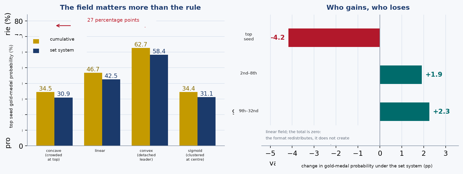
The first result is that the direction never changes. In all four fields, cumulative scoring takes the favourite to gold more often than the set system, and the gap always remains within the same narrow range:
fieldset / cumulative
concave30.9% / 34.5%
linear42.5% / 46.7%
convex58.4% / 62.7%
sigmoid31.1% / 34.4%
The difference lies between 3.3 and 4.3 percentage points across fields that otherwise look nothing alike. Six rounds do not amplify the single-match gap dramatically, nor do they erase it. The effect propagates through the bracket while remaining of the same general order of magnitude.
The second result is more interesting and is found in the left-hand values rather than in the between-format difference. Moving from a concave field to a convex one raises the favourite’s gold-medal probability from about 31% to 58%: a 27-percentage-point swing, compared with roughly four points separating the two scoring systems. Who else is in the competition matters almost ten times more than the arithmetic used to count the points. That observation belongs beside every debate about format: the sport pours enormous attention into a rule that shifts four percentage points, while field composition — effectively, who surrounds you in the competitive hierarchy — shifts twenty-seven.
The third result answers a question not yet asked: where do the four percentage points lost by the favourite go? A tournament still awards a gold medal, so probability does not disappear; it is redistributed. In the linear field, the top seed loses 4.2 percentage points, seeds 2–8 collectively gain 1.9, and seeds 9–32 gain 2.3. In other words, the set system transfers winning probability away from the favourite and towards outsiders, with a larger share going to the more distant group than to the immediate challengers.
This is not a new phenomenon in disguise. It is the same mechanism we have already seen twice, now viewed from the tournament level. A format that contains the damage from a poor arrow within the set in which it occurs protects the archer who makes the error; a format that is slightly less precise at identifying the better archer necessarily leaves more room for weaker archers to advance. Across a bracket, that protection becomes visible as a redistribution of winning probability, and the direction is exactly what one would expect: downward through the field.
Of all the findings in this study, this is the one closest to what the federation said it wanted in 2010: more open matches, less predictable outcomes, and more frequent upsets. On that dimension, the set system works, and it works for exactly the same reason that it discriminates slightly less well. These are two descriptions of the same property. Which description one values more is not a question a calculation can answer.
How many points are needed to know who is better?
So far we have treated the spread as if it were known. It is not. In fact, this part of the argument has some of the most practical consequences in the entire study and changes how a ranking table should be read.
A qualification round contains seventy-two arrows, and seventy-two arrows are a finite sample like any other. The resulting score is not the archer’s underlying ability; it is underlying ability plus the random variation of that particular session. The next question is therefore: how large is that random component?
The reason is already visible in the score-to-spread map and is worth making explicit. One qualification point corresponds to about seven tenths of a millimetre of spread, so two archers separated by three ranking points differ by less than two millimetres in the model. Asking seventy-two arrows to resolve a two-millimetre difference is asking too much. The answer can be calculated, and it helps to build towards it gradually. Take two truly identical elite archers — same group, same underlying precision, no real difference at all — and let each shoot seventy-two arrows, exactly as in qualification. The ranking gap that appears between them, generated entirely by chance and nothing else, averages about five points, and exceeds 6.5 points roughly one time in three. Not one or two points, as intuition might suggest between two people who are physically identical in the model.
| qualification gap | confidence in the true ordering |
|---|---|
| 1 point | 56% |
| 3 points | 68% |
| 5 points | 79% |
| 8 points | 90% |
| 12 points | 97% |
| 16 points | 99% |
A gap of a little over ten points is required before one can say, at the conventional 95% confidence level, which archer is genuinely more precise. Below about five points, much of what the ranking displays is noise. Whenever two adjacent archers in a tightly packed qualification table are separated by one, two, or three points — an entirely ordinary situation — their true relative ordering is largely unresolved.
Two points need to be made about these figures, and both strengthen the conclusion rather than weaken it. The first concerns what the calculation assumes we do not know. The confidence values are computed as if we had no prior information about the two archers — as if, before seeing their scores, every possible difference between their underlying expected scores were equally plausible. In a real competition field, however, nearby competitors in the ranking are usually also close in underlying ability. Taking that prior knowledge into account would make a given observed score gap even less conclusive than the table suggests. The second point is that the calculation includes only arrow-to-arrow random dispersion while holding each archer’s underlying form perfectly constant from the first shot to the last. It is the noise that would remain if the group itself were the only source of variation. Real competition adds everything the model ignores — sleep, shifting wind, day-to-day form, mental state — and most of those factors widen the uncertainty rather than narrow it. There is one important exception, because it acts in the opposite direction: a disturbance that affects both archers similarly — a wind change across the field, fading light — can partially cancel when one score is subtracted from the other, making the observed gap more informative rather than less. The net sign of all unmodelled effects is therefore an empirical question, not a mathematical consequence. Even so, individual-specific sources of variation are numerous, so the roughly five-point mean random separation and the ten-plus-point confidence threshold should be read as optimistic estimates of the true ambiguity in a qualification ranking.
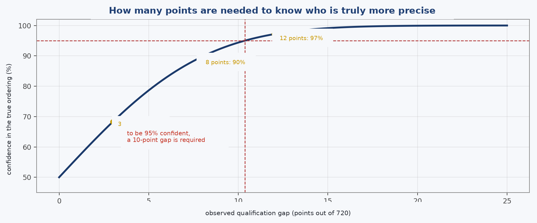
For a coach, this may be the most immediately useful result in the entire study, and it applies every time a ranking table is read. If your athlete finished fourth rather than second and only three points separate them from second place, that gap alone is not enough to establish a stable difference in precision. If the athlete finished twelfth rather than fourth and the gap is fifteen points, that is a signal worth investigating.
It also puts the debate that started this study back into proportion. Considerable attention is devoted to an arithmetic rule that changes outcomes by roughly two percentage points, while the instrument that determines who enters the bracket as the favourite — the qualification round — leaves the ordering of most closely matched pairs unresolved. The set system is a slightly coarse judge operating on an entry ranking that is much coarser still.
There is, however, a way out, and it does not require shooting better. It requires measuring more. The random variation in a single competition cannot be removed, but it can be diluted by averaging across multiple competitions, and the dilution is rapid: the variability of the mean falls with the square root of the number of rounds, so four competitions halve it and nine reduce it to one third. The practical question then becomes how many competitions are needed before and after a technical change for an improvement of a given size to become demonstrable.
The calculation is the same as before, applied to means rather than individual totals. For an archer scoring around 650, the required number of competitions per period is:
true improvementcompetitions per period
3 points29
5 points11
8 points5
10 points3
15 points2
The message is blunt but useful. A three-point gain over a season is excellent technical progress, yet demonstrating it requires roughly thirty competitions — in practice, about two seasons of data. A ten-point gain requires only three competitions per period. Between those two extremes lies the difference between a coach who evaluates a technical change from a block of measurements and one who evaluates it from the very next Sunday’s score.
Performance level again changes the picture. The same three-point improvement requires thirteen competitions rather than twenty-nine for a 690-level archer because that archer’s total score fluctuates less. The athlete who most needs to know whether progress is occurring — the one still changing many things — is also the athlete for whom the score responds most slowly.
This leads to a practical rule worth stating in full because it is the most immediate practical consequence of this section: a technical change should not be judged by short-term scores, because over the short term the score lacks the resolution to detect it. Judge the change through what can be observed directly — movement repeatability, group shape, video — and leave score, averaged over a sufficiently long block, to confirm months later that the change has reached the target.
What the model cannot see
The most important issue remains, and it concerns not what the model measures poorly, but what it deliberately does not measure at all.
Every number calculated so far rests on a model that is deliberately false. In the calculation, each arrow is independent of the previous one, always drawn from the same distribution, with no nerves, no fatigue, no momentum, no collapse. Skill is a single fixed quantity, unchanged from the first round to the final. It is a world of pure shooting mechanics in which the archer behaves like a machine repeating the same process.
Real archers are not like that, and nobody knows it better than someone who has competed. Bodies tighten as the stakes rise; rhythm is found and lost; a narrowly won set can ignite a comeback, while a set lost on one poor arrow can unravel everything that follows. Why, then, deliberately build a model that ignores exactly those effects?
Because that is how the invisible becomes visible. The model provides a baseline generated by precision alone: how many upsets would occur if archery were nothing but geometry and repetition. In the real world, there are more. And that difference — the gap between the number of surprises predicted by pure precision and the number actually observed — is not noise to be discarded. It is itself a measurable quantity: the contribution of everything the model deliberately leaves out.
The “mental game” — that vague thing everyone talks about and nobody can quite grasp — stops being vague in this framing. It becomes a residual: take the reversals observed in real competition, subtract those already justified by shooting precision alone, and what remains is the contribution of competitive pressure and other behavioural effects. The psychology of archery is no longer an aura surrounding performance; it is the distance between the model and the world, and that distance can in principle be quantified.
None of this is unique to archery. Every scoring format in every sport is, in one sense, a method for estimating a hidden quality, and questions of fairness can therefore be reframed as questions of measurement resolution. The same general machinery used here has been applied for decades to tennis and other racket sports. Archery is simply an unusually clean case because the latent quality is close to one-dimensional and its geometry is visible directly on the target. But transferability is a statement about method, not a result of this study: the calculations here concern 70-metre recurve and nothing else. Every other sport would require its own analysis from first principles, using its own geometry and rules.
Limitations
Three boundaries must be stated, because a number without its limitations is only half a truth.
The first is arrow independence. It is a modelling choice, not a description of real archers. It exists to isolate arithmetic from psychology, and the results should be read as a counterfactual — an answer to “what would happen if…”, calculated rather than imagined — not as a prediction of what will occur in competition. A set format can also reward different behaviours: protecting a set that is already secure, attacking when behind, managing rhythm differently. The model holds the arrows fixed and changes only the way they are counted. That is exactly what is needed to isolate the effect of the arithmetic, and exactly what prevents the model from predicting behaviour.
The second is idealised geometry. This is the limitation about which we can be most relaxed because it has been directly stress-tested: elliptical groups, shifted centres, and heavy tails either change the figure by only a few hundredths of a percentage point or reduce it by more than two thirds, without reversing the overall conclusion.
The third is the most important to state, and it is a design choice before it is a limitation. No calculation in this study uses any actually contested match. Everything follows from target geometry, published rules, and the dispersion model. This makes the conclusions general — they concern any pair of archers at a given level rather than one specific match — but it also means this work tells no story about any actual athlete, reconstructs no real tournament, and claims nothing about what happened on a particular occasion. It describes how the measurement instrument behaves, not what it measured in a given event.
What to take away
For athletes and coaches, several concrete lessons remain.
For the archer. Eliminating catastrophic shots remains one of the highest-value improvements, but for a different reason from the one people often imagine: it helps because it raises your score, not because the format rewards consistency. On this point, the calculation says the opposite of intuition, and we have already quantified it. At equal expected score, the set system favours the more erratic archer by roughly three percentage points because it contains the damage from a poor arrow within the set in which that arrow occurs. Do not expect the rules to reward you for being consistent; the reward for consistency is found in the score itself, not in the format. And do not treat a single loss to an equally matched opponent as a verdict on your ability: between near-equals, the coin is genuinely in the air for everyone.
For the coach. A match result is a noisy sample, not a judgement of ability. Even under the more discriminating of the two systems, the more precise archer loses regularly over a fifteen-arrow contest. The qualification ranking is noisy as well. Keep the most practically useful number in mind: below about a five-point gap over seventy-two arrows, the ranking says very little about the true ordering; below eight points, the evidence is still weak; and a confident conclusion requires a gap of a little over ten. A placing is not a verdict. It is an estimate with an error bar, and that bar is wider than any bracket makes visible. Evaluate an athlete’s development over many arrows, training averages, long rounds, and whole-season blocks — not over a single elimination match.
The distance between the group and the result
Taken together, the picture is sober. The set system is a slightly coarser measurement instrument than adding every point. Under the isotropic model, it costs roughly two to three matches per hundred in its ability to identify the more precise archer, and the cost becomes smaller at the higher performance levels where the format is actually used. It is not the lottery popular debate makes it out to be, but neither is it neutral. It represents a measured trade-off: a small loss of discrimination in exchange for robustness against catastrophic arrows — when anomalous shots are present, its disadvantage falls to less than one third — and for a match structure in which the damage from one bad arrow is contained within the set in which it occurs. Whether that trade-off is worthwhile is a decision for the sport, not for the model. The model can only say what the trade-off costs.
That cost comes entirely from the set rule, not from the match ending early. Forcing both archers to shoot all five sets does not change the winner at all, because the arrows saved by early termination are exactly those that could no longer affect the result. The price is paid by the score margin reset at every set boundary. And the paradox that frustrates spectators — winning despite a lower total score — occurs in roughly one match out of fourteen between equally matched archers, concentrated precisely where neither competitor had a materially stronger claim to victory.
But the result with the greatest practical weight is not about the match format. It concerns what comes before it. The qualification ranking, which establishes who is favoured and who meets whom, carries uncertainty much larger than the effect attributable to the arithmetic under debate. Two identical archers finish an average of five points apart by pure chance, and a gap of a little over ten points is needed before one can say with confidence who is better. The format is the visible and debated part of a mechanism whose roughest measurement stage is rarely examined. That disproportion is exactly the kind of thing explicit calculation can reveal.
And by subtraction, something larger remains. If this is the share of surprises that shooting geometry alone can justify, everything that occurs beyond it on the field — the champion eliminated in the first round, the impossible comeback, the collapse in the final set — belongs elsewhere. Technique is visible on the target, and we can now quantify it together with its uncertainty. The rest must be trained somewhere else. It is precisely in that distance between the group and the result that sport begins.
Note on data, sources, and method
This study uses no personal data of any kind, and none is needed. It contains no scores from real archers, refers to no completed competition results, names no athlete, and reconstructs no actual ranking. Every number follows from only three ingredients, all public and impersonal: target geometry as fixed by the rules; the rules of the two competition formats; and a mathematical model of shot dispersion.
The score levels cited — 692, 675, 665, and similar values — belong to nobody. They are reference points selected to place the reasoning within the range of real-world performance, in the same way a physics textbook might choose a one-kilogram mass. They make the calculations concrete; they do not describe any individual performance.
The only information taken from official international-federation documentation is regulatory in nature: the dimensions of the target and scoring rings, shooting distance, qualification-round and bracket structure, the operation of the set system and shoot-off, and the federation’s stated reasons for the 2010 format change.
The calculations are produced by the engine described in the dedicated chapter. The reproducibility package distributed with the study contains the mathematical specification for every equation, closed-form tests, a script that recalculates and checks every published value in these pages one by one, and the independent second implementation together with its comparison results. It declares the computational environment in which the reported numbers were frozen and is released under an open licence, so that anyone can repeat the calculations, challenge them, or extend them; anyone identifying an error can find contact details on the website. The competition rules were checked against the World Archery rulebook edition in force from 27 January 2026, in the updated version published on 13 March 2026, Book 3.
One substantive clarification follows from the calculations themselves rather than from any external concern. The section on uncertainty shows that a qualification score is a noisy indicator of the underlying precision of the archer who produced it. With the stated model and prior, score gaps below eight points — where confidence remains below 90% — do not provide strong information about the true ordering. A broader rule of caution follows: a score describes how that day went; it does not define the worth of the person who shot it, and it should not be used to judge them.
The main text shows only one equation: the one translating spread into the probability of scoring ten, nine, eight, and so on. That is deliberate. It is the only equation that needs to be seen in order to understand where the rest of the analysis comes from.
This appendix contains the twenty-four equations evaluated by the engine to produce every number printed in the study. They are presented as a complete translation of the underlying mathematics, with enough context for a reader who is not a professional mathematician to understand what each equation says, why it has that form, and what it cannot tell us. Readers interested only in recalculation can skip the prose and use the equations; readers interested in understanding how this kind of measurement works may find the prose the more useful part.
How each entry is structured
Each equation has at least four components. “In words” states what is being calculated without symbols. The equation displays it. “Where it comes from” reconstructs the derivation, usually in two lines. “A numerical example” applies it to a concrete case, most often the 690-level archer or the 692-versus-675 pair used repeatedly in the main text, so that every equation has at least one checkable value. Where necessary, a box lists what the equation does not cover: the boundaries beyond which it no longer applies.
At the end of each entry, the name of the function implementing it in the reproducibility package is provided.
Notation and units
The study moves across three units of measurement, and confusing them is the quickest way to obtain absurd numbers. Target geometry is expressed in millimetres on the target plane. The engine works in milliradians — angular units — because that makes the equations valid at any distance. The main text uses centimetres because that is the natural language in which archers think about group size. The bridge is simple: at seventy metres, one milliradian subtends seven centimetres.
| symbol | meaning |
|---|---|
| σ | spread of the group: the standard deviation of impacts along each axis. It is not the group radius and not the group diameter. |
| ρ, r | distance from the centre. ρ in milliradians; r in millimetres or centimetres. |
| w | width of one scoring ring: 61 mm, or 6.1 cm. |
| D | shooting distance, always 70 m in these pages. |
| F(ρ) | probability that an arrow lands within radius ρ. |
| pᵥ | probability that a single arrow scores exactly v points. |
| μ | expected score of one arrow; the expected 72-arrow total is 72μ. |
| S, T | score of an end (3 arrows) and of a round (72 arrows). |
| π_set, π_cum | probability that the more precise archer wins under the two formats. |
| Δ | format cost: the difference between the two win probabilities, expressed in percentage points. |
| Φ | cumulative distribution function of the standard normal distribution. |
The equations are meant to be read in order because each one uses what came before. The path is a single chain: target geometry leads to the probability of every arrow score; those probabilities lead to expected score; and inversion carries us back from score to spread. From there the two competition formats are constructed, and every published result follows from comparing them.
| group | contents |
|---|---|
| F01–F05 | Target geometry and the group model. How millimetres are converted to angles, what form the dispersion takes, and how to calculate the probability of landing within a given radius. |
| F06–F09 | The bridge between group and score, in both directions. This is where the equation shown in the main text appears. |
| F10–F15 | The two competition formats: the end, the set, the set match solved by backward induction, cumulative scoring, the shoot-off, and expected match duration. |
| F16–F21 | The quantities reported in the main text: format cost, set margins, the early-stopping theorem, the paradox rate, and qualification noise. |
| F22–F24 | Robustness tests and tournament calculations: deformed groups, increased central density, parametric fields, and propagation through the bracket. |
Five equations establish two things: how the target is constructed, and how an arrow group is represented mathematically.
F01 · Target-face geometry
In words. The 70-metre target is a 122-centimetre disc divided into ten concentric scoring rings of equal width. That uniformity is what makes the rest of the mathematics simple: the ring boundaries are not a list of unrelated numbers, but multiples of a single width.
rₖ = w · k, k = 1, …, 10 vₖ = 11 − k
w = 61 mm rₓ = 30.5 mm
Where it comes from. The outer radius of ring k is k times the ring width w. The score assigned to that ring is 11 minus k: the first ring is worth ten, the second nine, and so on down to the tenth, worth one. At the centre is an additional circle of radius 30.5 mm, exactly half a ring width, called the X ring. It still scores ten and is used to break ties.
A numerical example. The ten ring has a radius of 6.1 cm; the nine extends to 12.2 cm; the outer edge of the target lies 61 cm from the centre. An elite archer’s spread is roughly three quarters of the width of a single scoring ring. That disproportion is part of what makes archery what it is.
F02 · Angular scale
In words. An arrow group has no truly absolute size; it has an angular size. The same aiming error produces a group twice as wide at twice the distance. By working in angles rather than centimetres, the equations remain valid at any distance without being rewritten.
ρ = r / D at 70 m: 1 mrad = 7 cm
Where it comes from. A milliradian is one thousandth of a radian, and for small angles one radian at distance D subtends D units of length. Therefore, at a distance of D metres, one milliradian subtends D millimetres: at seventy metres, seventy millimetres, or seven centimetres. Dividing a length in millimetres by distance in metres gives milliradians directly.
A numerical example. A 61 mm ring width at seventy metres is 61/70 = 0.871 mrad. The X ring radius is 30.5/70 = 0.436 mrad. A 690-level archer has σ = 0.637 mrad, equivalent to 4.46 cm.
F03 · Dispersion model
In words. Where an arrow lands is the result of many small, partly independent inaccuracies — draw, release, air movement, execution — adding together. When many small independent causes are summed, their combined effect tends towards a Gaussian distribution. The group is therefore modelled as a two-dimensional bell-shaped distribution centred on the aiming point. The model can add a second, wider component with low weight to represent anomalous arrows: shots that an ordinary Gaussian core would not explain well.
(X, Y) ~ (1−ε) · N(b, Σ) + ε · N(b, k²Σ)
Σ = diag(σₓ², σᵧ²)
Where it comes from. The first component represents ordinary execution, with horizontal spread σₓ and vertical spread σᵧ, centred at b. The second has the same shape but is k times wider and carries weight ε. Setting ε = 0 leaves the simple Gaussian; additionally setting σₓ = σᵧ and b = 0 gives the centred circular case used throughout most of the study because it has an exact solution.
A numerical example. The four configurations examined in the study are: a centred circular group (the baseline); a vertical ellipse with σᵧ = 1.5σₓ; a group shifted 3 cm from the centre; and a heavy-tailed model with ε = 0.05 and k = 3, meaning one arrow in twenty is drawn from a group three times wider.
What it does not cover
σ is the standard deviation along each axis, not the radius of the group and not its diameter. Confusing these quantities is the most common error when interpreting dispersion figures and changes the scale by a factor of two or three.
The model assumes arrows are independent. An archer who loses control for three consecutive shots violates this assumption, and the main text lists this explicitly among its limitations.
F04 · Probability of landing within a radius
In words. This is the equation that makes the rest of the model work. Given the spread of the group, what is the probability that an arrow lands inside a circle of specified radius? In the centred circular case, the answer is a single exponential, which is why the model remains analytically tractable.
centred circular: F(ρ) = 1 − exp( −ρ² / 2σ² )
shifted group: F(ρ) = 1 − Q₁( ν/σ, ρ/σ )
Where it comes from. If the two impact coordinates are independent Gaussian variables with the same spread σ, radial distance from the centre follows a Rayleigh distribution, and the probability of exceeding radius r is exactly exp(−r²/2σ²). This equation appears wherever two independent perpendicular error components are combined — in ballistics, radar, metrology, and many other fields. The probability of landing within r is simply its complement to one.
When the group is shifted from the centre by an amount ν, the radial distribution becomes a Rice distribution and the exact expression involves the Marcum Q-function: it remains exact but is no longer elementary. When the group is elliptical, circular symmetry is lost and no elementary antiderivative exists; the probability must then be evaluated numerically in polar coordinates:
F(ρ) = ∫₀^{2π} ∫₀^{ρ} (2πσₓσᵧ)⁻¹ ·
exp[ −(t cosθ − bₓ)²/2σₓ² − (t sinθ − bᵧ)²/2σᵧ² ] · t dt dθ
mixture: F(ρ) = (1−ε) F_{σ}(ρ) + ε F_{kσ}(ρ)
The important detail. The factor t at the end of the integral is the Jacobian for the transformation to polar coordinates: it accounts for the fact that a thin annulus farther from the centre contains more area than one close to the centre. Omitting it is the most natural mistake in this calculation, and it produces values that can look plausible while being wrong. This is precisely why the main text describes validation against a very large random sample: in the circular case, the angular component simplifies away, so agreement with the exact circular formula alone would not be enough to expose that error.
A numerical example. For the 690-level archer, with σ = 4.46 cm, the probability of landing outside the ten-ring boundary is exp(−6.1² / 2·4.46²) = 0.393. In other words, almost four arrows out of ten fall outside the inner yellow ring. In the circular case, the numerical integration reproduces the exact expression to the eleventh decimal place.
F05 · How large is that group, in practical terms?
In words. σ is convenient in equations but not especially intuitive for an archer. These three conversions translate it into quantities visible on the target: the mean distance of an arrow from the centre, the median distance, and the radius containing 95% of arrows.
E[R] = σ √(π/2) ≈ 1.253 σ median = σ √(2 ln 2) ≈ 1.177 σ
R₉₅ = σ √(2 ln 20) ≈ 2.448 σ
Where it comes from. These are the moments and quantiles of the Rayleigh distribution from F04. The quantile follows by inverting the exponential: to find the radius containing a fraction q of arrows, set 1 − exp(−r²/2σ²) = q and solve, giving r = σ√(−2 ln(1−q)).
A numerical example. For a 690-level archer, σ = 4.46 cm: the mean arrow lands 5.59 cm from centre, half of all arrows fall within 5.25 cm, and 95% fall within 10.92 cm. That last number is less than two ring widths: almost the entire group of an elite archer lies inside the nine.
This is the pivot of the entire study. A score is public information: it appears in results and anyone can read it. Spread is not; it requires measuring the landing position of every arrow, and such coordinate data are generally not publicly available. These four equations build the bridge between the two, allowing us to reason about archers using a number that everyone can observe.
F06 · Probability of each individual score
In words. This is the equation shown in the main text. It gives the probability that an arrow scores exactly s points: take the probability of landing inside the outer boundary of the ring and subtract the probability of landing inside the inner boundary. Two subtractions produce the archer’s complete single-arrow score profile.
pᵥ = F(ρᵥ) − F(ρᵥ₋₁) p₀ = 1 − F(ρ₁₀)
in the centred circular case, for s = 1 … 10:
P(S = s) = exp( −[(10−s)w]² / 2σ² ) − exp( −[(11−s)w]² / 2σ² )
Where it comes from. The ring worth s points lies between an inner radius of (10−s)w and an outer radius of (11−s)w; this follows from F01 by substituting k = 11−s. Scoring exactly s means landing outside the inner boundary but not outside the outer one. Because exp(−r²/2σ²) is the probability of lying beyond radius r, the difference between the two exponentials is exactly the required probability. Writing the expression as two exponentials rather than two “one minus” terms is not cosmetic: it is the same algebra after the ones cancel.
A check. For s = 10, the inner radius is zero, so the first exponential equals one and the expression becomes 1 − exp(−w²/2σ²), exactly the probability of landing inside the first scoring ring. This sanity check makes the rest of the formula easy to read.
A numerical example. For a 690-level archer with σ = 4.46 cm: ten is scored 60.73% of the time, nine 36.89%, eight 2.36%, seven about two times in ten thousand, and lower scores essentially never. Summing over s = 1 to 10 gives exactly one, as it should. The engine, which evaluates the general geometry numerically, returns the same probabilities with a discrepancy below 10⁻¹⁷.
What it does not cover
A miss is not included in the s = 1 … 10 expression. For s = 0 there is no outer scoring-ring boundary to subtract; the probability is simply exp(−(10w)²/2σ²).
The X ring is not covered by the scoring-ring formula above. Its radius is half a ring width rather than an integer multiple of w, so it does not fit the (11−s)w scheme. F09 is used instead.
The closed form applies only to centred circular groups. Elliptical, shifted, and heavy-tailed groups require the general integral in F04.
The arrow is treated as a point. Under the rules, an arrow touching a scoring line receives the higher value, which is equivalent to expanding each scoring boundary by the radius of the shaft. If this were included, the same σ would produce 691.2 rather than 690. The simplification does not change the conclusions because σ is never measured directly; it is calibrated from score, so the geometric change is absorbed into calibration. It does, however, shift the quoted centimetre values by about 2%.
F07 · Expected score
In words. Once the probability of every score is known, the mean score of one arrow is simply the probability-weighted average of those values. Multiplying by seventy-two gives the expected total for a qualification round.
μ(σ) = Σ_{v=0}^{10} v · pᵥ(σ) T(σ) = 72 · μ(σ)
Where it comes from. This is just the definition of expected value applied to the score probabilities in F06. Nothing more is required.
The property that matters. μ is strictly decreasing in σ over the entire relevant domain: every spread corresponds to one expected score, and the tighter the group, the higher the score, with no reversals. This sounds obvious but is not guaranteed by every possible target geometry. That monotonicity is what makes F08 possible.
A numerical example. At σ = 4.46 cm, the mean is 9.5833 points per arrow, or 690 over 72 arrows. At σ = 7.17 cm, it falls to 9.0278, or 650.
F08 · Calibration: from score to spread
In words. This is F07 read in reverse. Given an expected score, what is the unique spread that produces it? This equation is what allows the model to discuss real-world performance levels without having impact-coordinate data: begin with a score, derive a group, and calculate everything else from there.
σ(μ̄): the unique solution of μ(σ) − μ̄ = 0
Where it comes from. There is no explicit inverse formula: μ(σ) is a sum of exponentials and cannot be inverted algebraically. The root is found numerically using Brent’s method to a tolerance of 10⁻¹⁰. Uniqueness is guaranteed by the monotonicity established in F07: a strictly decreasing function crosses any admissible value only once.
A numerical example. An expected 72-arrow score of 690 gives σ = 4.4613 cm; 692 gives 4.3259 cm; 650 gives 7.1654 cm. Across the range of interest the relationship is almost perfectly linear: one point corresponds to roughly 0.68 mm of spread, and that conversion remains almost unchanged from 630 to 700.
What it does not cover
The input is expected score, not an observed score from one competition. An archer who scores 690 in a particular round does not necessarily have an underlying expected score of 690. That round is a single draw from the performance distribution, and its standard deviation is 4.58 points. An observed 690 is therefore compatible, at 95% confidence, with a spread anywhere from roughly 3.85 to 5.07 cm — an interval more than a centimetre wide. Inferring the group from a single competition is an estimation problem with uncertainty, not a simple inversion. F21 quantifies that uncertainty.
F09 · X ring rate
In words. The X ring is simply another circle, only smaller. Its probability is obtained from the same radial formula using the X ring radius.
ρₓ = rₓ / D P(X) = 1 − exp( −ρₓ² / 2σ² )
Why it deserves its own entry. The X radius should be derived from target geometry rather than hard-coded as an independent constant. That may sound pedantic, but it is not. If target geometry or shooting distance changes, a hard-coded value can silently remain at the old setting and produce percentages that no longer correspond to the target being analysed.
A numerical example. At seventy metres, ρₓ = 30.5/70 = 0.4357 mrad, equivalent to 3.05 cm. A 692-level archer places 22.0% of arrows in the X ring: 15.8 out of 72. The same archer scores 45.4 tens.
So far we have described one archer. Now we place two archers against one another and calculate who wins under each arithmetic system. Six equations are enough, and none requires a match to be simulated: the complete probability is constructed by enumerating and weighting all possible ways the match can unfold.
F10 · Score of an end
In words. If the probability of every one-arrow score is known, the probability of a particular three-arrow total is obtained by counting all combinations that produce that total. The operation that performs this calculation is convolution.
P(Sₙ = s) = (p^{*n})ₛ s = 0, …, 10n
Where it comes from. With two arrows, the probability of scoring 19 is the probability of 10 then 9 plus the probability of 9 then 10: sum every pair whose values add to 19, multiplying the corresponding probabilities. Repeating this for every possible total gives the two-arrow distribution; applying the same operation again gives the three-arrow distribution. That is exactly convolution, and with only eleven possible scores per arrow the computation is straightforward.
A numerical example. A set uses three arrows, so the total ranges from 0 to 30. The cumulative comparison uses fifteen arrows, so the range is 0 to 150. The 692-level archer shoots a perfect 30 in 25.0% of ends; the 675-level opponent does so in 9.9%.
What it does not cover
Convolution assumes arrows are independent: the outcome of one arrow does not alter the distribution of the next. This is the strongest assumption in the study and is explicitly listed among the model limitations. If errors occurred in clusters — three poor arrows in succession rather than three isolated errors — the set system would tend to benefit because the cluster would be contained within one set.
F11 · Who wins an end?
In words. Given the end-score distributions for both archers, three probabilities follow: the first archer scores more, the two tie, or the first scores less. The entire set match is built from these three numbers.
p_w = Σₛ aₛ · Bₛ₋₁ p_t = Σₛ aₛ · bₛ
p_l = 1 − p_w − p_t
Where it comes from. For every score s that A can produce, multiply A’s probability by the probability that B scores strictly less — B’s cumulative probability through s−1. Summing across all s gives the probability that A wins the end. The tie probability is the sum of products for equal scores. Loss is calculated as the residual, which guarantees that the three probabilities sum exactly to one.
A numerical example. For 692 versus 675, the stronger archer wins an end 55.5% of the time, ties 24.7%, and loses 19.8%. The tie probability is strikingly high — about one end in four — and matters greatly in a format that awards set points.
F12 · The one-arrow shoot-off
In words. When a match remains tied, each archer shoots one arrow and the arrow closest to the centre wins. This equation gives the probability that the more precise archer wins that shoot-off, and the expression is unexpectedly simple.
p_so = σᴃ² / ( σᴀ² + σᴃ² )
Where it comes from. For a centred circular Gaussian group, squared radial distance from the centre follows an exponential distribution with mean 2σ². For two independent exponential variables, the probability that the first is smaller than the second is the second rate parameter’s contribution relative to the sum; after substitution this reduces exactly to σᴃ²/(σᴀ²+σᴃ²). No approximation and no numerical integration are required.
Why it is notable. Under these assumptions, the rule “closest to the centre wins” is statistically optimal: among all decision rules that could be applied to a single arrow from each archer, it maximises the probability of identifying the more precise archer.
A numerical example. Between 692 and 675, the shoot-off is not a coin toss: the stronger archer wins it 61.57% of the time. This may look like a minor detail, but it is not. Replacing that value with 0.5 shifts paradox rates by about half a percentage point, and this was one of the errors detected and corrected during validation.
What it does not cover
All three assumptions — circular groups, centred groups, and independent arrows — are required. For elliptical or shifted groups, the closed form is not valid and the general integral form is used instead; in the circular case, that integral reproduces the same value.
F13 · The set match, solved backward
In words. This is the equation that calculates a competition that was never played. The idea is to start at the end: every state in which the match can terminate already has a known winner. Move backward one set, and the probability of eventually winning from that state is the weighted average of the probabilities following the three possible set outcomes. Repeat until the initial 0–0 state is reached, yielding the exact match-win probability.
V = 1 if a ≥ 6 V = 0 if b ≥ 6
V(a,b,5) = 1 if a > b ; 0 if b > a ; p_so if a = b
V(a,b,e) = p_w V(a+2, b, e+1)
+ p_t V(a+1, b+1, e+1) + p_l V(a, b+2, e+1)
π_set = V(0, 0, 0)
Where it comes from. A match state is described by three numbers: A’s set points, B’s set points, and the number of sets already played. From each state there are three possible transitions — A wins the set and gains two points; the set is tied and each gains one; B wins and gains two — with the probabilities from F11. The probability of ultimately winning from a given state is therefore the weighted sum of the winning probabilities from the three successor states. This procedure is backward induction, the same general method used to solve finite games with known transition structure.
An easy implementation trap. Set-point totals can be odd because a tied end awards one point to each archer. Reachable states therefore include 1–1, 3–1, 3–3, 5–3, and 5–5. An implementation that considered only even scores would produce incorrect values without necessarily signalling an error. The 5–5 state is the only terminal end-of-five-sets state that does not decide the match; it proceeds to the F12 shoot-off.
A numerical example. The 692-level archer beats the 675-level archer under the set system with probability 0.846819. The calculation is exact: there is no sampling and no simulation, and repeating it returns the same value to the last calculated decimal place.
F14 · Cumulative scoring
In words. The alternative arithmetic is straightforward: add all arrow scores and award the match to the higher total, with the same shoot-off if totals are tied. The equation is simpler than the set-match recursion because there are no internal set states to traverse.
π_cum(n) = P(Tᴀ > Tᴃ) + p_so · P(Tᴀ = Tᴃ)
Where it comes from. The two total-score distributions are obtained from F10 using n arrows. The probability that A’s total exceeds B’s is calculated as in F11, now over match totals rather than three-arrow ends. Exact ties are resolved by the same shoot-off used in the set format. This is essential: otherwise the comparison between formats would mix the aggregation effect with a difference in tie-breaking rules.
A numerical example. Over fifteen arrows, the 692-level archer beats the 675-level archer with probability 0.870019, compared with 0.846819 under the set system. The difference between those two values is the format cost — the central quantity this study is designed to measure.
F15 · Expected match length
In words. A set match can end after three, four, or five sets. This equation gives the expected number of sets played and therefore the expected number of arrows actually shot.
E[set] = Σ_{k=1}^{5} k · πₖ n̄ = 3 · E[set]
Where it comes from. πₖ is the probability that the match ends exactly at set k, returned as a by-product of the F13 recursion. The probability mass entering absorbing states at each depth is accumulated, and the expected value follows directly.
A numerical example. Between 692 and 675, the expected match length is 4.268 sets, or 12.80 arrows rather than the full fifteen. That difference of just over two arrows is the quantity examined in the F19 decomposition and the F18 early-stopping theorem.
Everything claimed in the main text comes from these six equations. The first two measure the cost of the format and the information it discards; the third is a theorem identifying where that cost does and does not originate; the final three concern the paradox rate and the amount of noise in qualification rankings.
F16 · Format cost
In words. This is the central quantity of the study: how much more often cumulative scoring identifies the correct winner than the set system when the comparison is made at equal arrow count. It is measured in percentage points: matches per hundred.
Δ(Tᴀ, Tᴃ) = 100 · [ π_cum(15) − π_set ]
Where it comes from. It is simply the difference between F14 and F13. Two choices make the comparison fair: the same fifteen-arrow maximum in both formats, justified by the theorem in F18; and the same shoot-off rule, so that the difference isolates aggregation rather than different tie-breaking procedures.
How to read the sign. A positive value means cumulative scoring more often identifies the more precise archer. If both archers have the same expected score, there is no more precise archer to identify: both formats produce a 0.5 win probability and Δ is zero by symmetry, not because either format has succeeded. This distinction matters. A zero at equality does not mean “the two formats are equally good”; it means the discrimination question has no object at that point.
The convention. Format cost depends on which opponent is placed against the stronger archer, so a criterion is needed. Here the stronger archer’s level is fixed, the opponent is varied on a half-point grid down to forty points lower, and the maximum difference is reported. This is a worst-case measure, not an average-case one. It is a conservative convention and must be stated because a different convention would produce a different number.
A numerical example. At a stronger-archer level of 692, peak cost is 2.32 percentage points, occurring against an opponent around 675. At lower performance levels the cost rises: 2.38 at 690, 2.63 at 680, 2.82 at 670, and 2.97 at 660. The set format penalises more as the absolute level moves farther from the elite.
F17 · By how much is a set won?
In words. The set system awards two points for a set victory whether the margin is one point or ten. This equation measures the average size of that winning margin: the information cumulative scoring preserves and the set format erases.
E[δ | δ > 0] = Σ_{d>0} d · P(δ = d) / P(δ > 0)
Where it comes from. δ is the difference between the two archers’ end scores. Its distribution is obtained from the two F10 end distributions by cross-correlation — equivalently, convolution of one distribution with the reversed version of the other. The conditional mean is then taken over positive values only.
A numerical example. Between 692 and 675, a won set is won by an average of 1.76 points, and by two or more points in more than half of all cases. Between identical archers, the average winning margin falls to 1.41. Whatever its size, that margin is compressed into the same two set points and does not cross the set boundary. In one line, that is the mechanism behind the entire format cost.
F18 · Theorem: early stopping is free
In words. A set match stops as soon as one archer reaches six set points, so the remaining arrows are not shot. It is natural to think that those missing arrows must reduce measurement precision. This theorem shows that they do not: the archer who wins under early stopping would also win if the match were always played to completion. Always — not merely on average.
Statement. Compare two ways of playing the same match. The first is the regulation format: stop as soon as one archer reaches six set points, leaving the remaining arrows unshot. The second always plays all five sets, then awards the match to the archer with more set points, resolving 5–5 with the same shoot-off. The theorem states that the two procedures always identify the same winner. Not on average, and not almost always: for every pair of archers and every individual match realisation, one by one.
Proof. Across five sets, a total of ten set points is distributed, two per set. Suppose A reaches six at the end of set e. Since 2e set points have been awarded by then:
bₑ = 2e − aₑ ≤ 2e − 6
Across the 5−e remaining sets, another 2(5−e) points can be distributed. Even if every one goes to B, B’s final total cannot exceed:
b₅ ≤ (2e − 6) + (10 − 2e) = 4
while A has at least six. Therefore a₅ ≥ 6 > 4 ≥ b₅: A also wins the full-length version. The argument is symmetric for B, and if neither archer reaches six before the fifth set the two procedures coincide by construction. The theorem is established without any numerical calculation: it is a property of set-point arithmetic, not of the dispersion model.
Verification. The engine evaluates both versions for the 692-versus-675 pair and obtains 0.846819200346337 in both cases. The difference is not merely small; it is exactly zero.
Why it matters. There are two consequences, and they are among the most important in the study. First, the correct comparator for F16 is fifteen-arrow cumulative scoring, not cumulative scoring over the 12.8-arrow average match duration. Second, and directly following from the first, the entire format cost belongs to the aggregation rule rather than to early stopping. If short duration were the cause, lengthening the match would reduce the gap. The opposite occurs: three sets versus nine arrows produce a 1.84-percentage-point gap, five versus fifteen produce 2.32, and seven versus twenty-one produce 2.38. Every additional set adds another boundary at which score margin is discarded.
F19 · Decomposition
In words. The total difference can be decomposed by comparing the set system with two cumulative-score references: fifteen-arrow cumulative scoring and cumulative scoring evaluated at the set match’s average effective duration. The second component must be labelled carefully.
π_cum(n̄) = π_cum(⌊n̄⌋) + (n̄ − ⌊n̄⌋) · [ π_cum(⌊n̄⌋+1) − π_cum(⌊n̄⌋) ]
Δ_rule = 100 [ π_cum(n̄) − π_set ] = 0.50 pp
Δ_extra_arrows = 100 [ π_cum(15) − π_cum(n̄) ] = 1.82 pp
Where it comes from. The average duration from F15 is not an integer — 12.80 arrows — while cumulative scoring is defined only for integer arrow counts, so the value is obtained by linear interpolation between twelve and thirteen arrows.
The label. The second term is not the “cost of short match length.” F18 proves that early stopping itself costs exactly zero. The term measures something different but still meaningful: the marginal discriminative value of the additional 2.2 arrows under cumulative scoring — in other words, how much extra information an additional arrow contributes when all points are retained. It is a legitimate quantity that, for a while, carried the wrong name.
Why not average over match durations? It might seem natural to calculate cumulative performance by averaging across the distribution of observed set-match lengths rather than evaluating at the mean length. That would be wrong: match length is correlated with outcome structure — highly imbalanced contests tend to finish earlier — so weighting by duration would reintroduce exactly the information the comparison is intended to isolate. For transparency, rounding to thirteen arrows would raise the first term to 0.68, while averaging across the duration distribution would lower it to 0.32.
F20 · The paradox: winning with fewer points
In words. Under the set format, the match winner can finish with fewer raw points than the opponent. This equation calculates how often that occurs.
κ⁺(d) = P(δ = d), d > 0 κ⁻(d) = P(δ = d), d < 0 p₀ = P(δ = 0)
Where it comes from. The recursion is the same as in F13, but the state carries an additional quantity: the cumulative raw-score difference between the archers. The sign of δ determines who wins the set and therefore how set points advance; the magnitude of δ updates the raw-score difference. At terminal states, the probability mass in which the match winner has a negative raw-score difference is summed. Match state and raw-score margin must therefore be propagated together, which is why a joint recursion is required rather than two separate calculations.
Two definitions. The paradox can be measured in two ways, answering different questions. The first compares totals over the arrows actually shot — nine, twelve, or fifteen depending on the match path. The second compares both archers over fifteen arrows as a counterfactual: “if all five sets had been completed, who would have had the higher raw total?” The second definition assumes that the unshot arrows would have been independent continuations of the same stochastic process, and that assumption is stated explicitly.
A numerical example. For essentially equal elite archers — 692 versus itself — the paradox occurs in 7.1% of matches when calculated over arrows actually shot and 7.6% under the fifteen-arrow counterfactual. The rate rises at lower levels: 9.2% at 670 and above 10% at 650. For the peak-cost pair, 692 versus 675, where the shoot-off is asymmetric, the corresponding values are 4.7% and 5.2%, lower because the underlying skill difference makes reversals harder.
F21 · How much noise is there in a qualification score?
In words. A 72-arrow qualification round is not an exact measurement of ability; it is one sample. These equations quantify how far apart two identical archers can appear in the ranking purely by chance, and how much confidence can be placed in an observed score gap.
v = Σᵥ (v − μ)² pᵥ SD(T) = √(72 v)
SD(D) = √2 · SD(T) E|D| = SD(D) · √(2/π)
Where it comes from. The variance of one arrow is obtained from its score distribution. For seventy-two independent arrows, variances add, so the standard deviation of the total is the square root of seventy-two times the one-arrow variance. For the difference between two independent rounds, the variances add again, giving the √2 factor. The expected absolute difference — the gap a reader sees in a ranking — is a different quantity again: for a zero-mean normal variable it equals √(2/π) times the standard deviation, about 79.8% of it.
A numerical example. At a 692 performance level: one-arrow variance is 0.2757; the standard deviation of a 72-arrow round is 4.455 points; the standard deviation of the difference between two such rounds is 6.300; and the mean absolute gap is 5.027. The values 6.30 and 5.03 describe related but distinct quantities and are not interchangeable. Preventing that confusion is one reason for spelling the derivation out here.
The observed gap corresponding to 95% one-sided confidence in the true ordering is 1.645 times the standard deviation of the difference: 10.36 points. From this follows the confidence table:
| observed gap | confidence in the true ordering |
|---|---|
| 1 point | 56.3% |
| 3 points | 68.3% |
| 5 points | 78.6% |
| 8 points | 89.8% |
| 12 points | 97.2% |
| 16 points | 99.4% |
What that column represents. It is not a frequentist confidence interval; it is a posterior probability. Let Δ be the true difference in expected scores and g the observed difference. Then D | Δ ~ N(Δ, SD(D)²). Assuming that, before observing the scores, all values of Δ are equally plausible, the posterior distribution is N(g, SD(D)²), and:
C(g) = P(Δ > 0 | D = g) = Φ( g / SD(D) )
What it does not cover
The prior matters and must be named. “All values equally plausible” does not identify a distribution unless one specifies which quantity is assigned a flat prior: spread, expected score, and log spread lead to different posterior tables. Here the prior is flat on the difference between expected scores.
The direction of the bias is known. In a real competition field, archers who appear close in the ranking are also more likely to be close in underlying ability, so a realistic prior would make an observed score gap less conclusive than the table above suggests. These figures are deliberately optimistic.
The final three equations answer the question a sceptical reader is right to ask first: what if the assumptions are wrong? Change the shape of the group, change its central concentration, change the composition of the competitive field, and see whether the conclusion survives.
F22 · Comparing two shapes without comparing two skill levels
In words. To determine whether group shape changes the result, shape must be changed while everything else is held constant. The problem is that deforming a group also changes expected score. Without recalibration, one ends up measuring how good the archer is rather than the effect of group shape.
s*(μ̄) : the unique s such that μ( M(s) ) = μ̄
Where it comes from. This is another inversion like F08, now applied to a family of group shapes rather than to a single spread. Given a target mean score, the scale parameter that produces that score under the chosen shape is found numerically. Once this is done, every compared shape generates the same expected score and any remaining difference can be attributed to shape alone.
Why it matters. A 692-level group stretched to 1.5:1 without recalibration actually corresponds to about 675.2 points. The deformation would have degraded the archer by 17.3 points without any explicit warning, and one could wrongly conclude that shape matters enormously when in fact a strong archer had simply been compared with a much weaker one. With recalibration, shape is almost irrelevant: circular 2.32 percentage points, ellipse 2.34, shifted group 2.36.
The one shape that materially changes the result. The heavy tail: with one arrow in twenty drawn from a group three times wider, format cost collapses to 0.68 percentage points, less than one third of baseline. The set system protects the archer who makes an extreme error because the catastrophic arrow is contained within the set where it occurs. The weakness becomes a shield, and a shield necessarily protects someone.
Mixture convention. When recalibrating the heavy-tailed model, both components are scaled together while preserving the fixed 3:1 spread ratio between tail and core. This is a modelling choice, it must be declared, and it is not neutral: rescaling only the core would produce a much lower value.
Consistency, quantified. Compare a consistent and an inconsistent archer who produce the same mean score. The consistent archer wins 48.5% of matches under cumulative scoring but only 45.4% under the set system. In this construction, the set format penalises consistency, contrary both to common intuition and to one of the stated reasons for its adoption.
What it does not cover
In the deformed-group models, shoot-offs are evaluated using the equivalent circular spreads. Otherwise group shape would re-enter through the tie-break precisely at the point where the robustness comparison is intended to isolate it.
F23 · What if the group is more concentrated at the centre?
In words. A reasonable objection is that elite archers may have a more concentrated central core than a simple Gaussian predicts. This equation constructs groups with that property, while holding expected score fixed, and tests whether the conclusion remains stable.
F(ρ) = (1−w)[1 − exp(−ρ²/2s₁²)] + w[1 − exp(−ρ²/2s₂²)]
Where it comes from. Two circular components of different spreads are mixed with equal weights. The parameters s₁ and s₂ are not chosen arbitrarily; they are determined by two constraints: preserving the target mean score and reaching the desired X ring rate. Increasing the X rate while holding mean score fixed produces exactly the intended geometry — greater density at the centre together with a more dispersed outer component.
The convention. Both archers are given the same increment above the X rate their baseline circular group would naturally produce. At zero increment, the mixture collapses back to the pure circular model and the cost returns to the F16 peak. This is the consistency check showing that the construction is properly anchored.
A numerical example. Raising the stronger archer’s X rate from 22% to 30% increases format cost from 2.32 to 3.13 percentage points: 2.53 at 24%, 2.74 at 26%, and 2.94 at 28%. The direction — greater central concentration increases the cost by roughly 0.8 percentage points across this deliberately wide perturbation — is robust to the exact admissible construction. The precise intermediate values are not, which is why the convention must be stated.
F24 · Parametric fields and bracket propagation
In words. A tournament is not one match; it is a six-round tree of sixty-four archers. To determine whether format changes tournament winners, a field must be constructed and match probabilities propagated round by round. The fields used here are not empirical fields. They are four deliberately chosen shapes designed to isolate how the distribution of performance levels affects the result.
Tᵢ = 684 − 60 · f(u), u = (i−2)/62
f: concave u^{1.6} · linear u · convex u^{0.6} · logistic sigmoid
Where it comes from. The top and bottom of the field are held fixed — the top seed at 692, the second seed at 684, and the last at 624 — while only the function filling the space between them changes. A concave field clusters many archers near the top; a convex field has fewer near the elite and a long lower tail; the linear field spreads them uniformly; the sigmoid field concentrates them around the middle. Each score is converted to spread using F08, pairwise match probabilities are calculated with F13 and F14, and those probabilities are propagated through the standard seeded bracket pairing 1 with 64, 32 with 33, and so on.
A numerical example. Top-seed gold-medal probability, set format versus cumulative: concave field 30.9% versus 34.5%; linear 42.5% versus 46.7%; convex 58.4% versus 62.7%; sigmoid 31.1% versus 34.4%. Field composition matters more than scoring format — the concave-to-convex difference is twenty-seven percentage points — but the direction of the format effect is the same in all four cases.
What it does not cover
None of these fields represents a real competition field. They are parametric constructions used to show that the conclusion does not depend on one particular composition, not to predict the outcome of any future tournament.
Every equation in this appendix rests on modelling choices. Listing them together at the end is useful for readers who want to know not merely whether the calculations are correct — those can be repeated — but whether the model is describing the right thing. Where the direction can be inferred, the third column indicates how the result would be expected to move if the assumption failed.
| assumption | why it is used | if it fails |
|---|---|---|
| Independent arrows | Makes total-score distributions convolutions and allows exact calculation. | With clustered errors, the set system gains an advantage because the bad shots become concentrated within a single set. |
| Constant dispersion within the round | Allows one parameter per archer; no data are available to estimate within-round drift. | Qualification uncertainty widens: the F21 thresholds become a floor, not a ceiling. |
| No dependence between the two archers | Excludes shared wind and mutual influence. | Shared wind reduces the variance of the score difference, making an observed gap more informative. |
| No strategy and no shooting-order effect | The model measures precision, not game behaviour. | Direction unknown: this belongs to the unexplained residual. |
| No pressure effect | Cannot be quantified without data. | Not identifiable: the residual would also contain model error, equipment effects, and day-specific form. |
| Synthetic performance levels | No real archer’s score enters the study. | Not applicable: the conclusion concerns the format, not a population. |
| Bivariate Gaussian family | Analytically tractable and stress-tested against three deformations. | Tested: ellipse and bias shift the cost only by hundredths of a percentage point; a heavy tail reduces it to less than one third. |
| Parameters treated as known without uncertainty | The two archers are defined by their expected scores. | If spread must be estimated, parameter uncertainty adds to format uncertainty (see F08 and F21). |
| Point-like arrow | Simplifies scoring-zone geometry. | The line-cutter rule shifts the score-to-spread map by roughly one point; the effect is absorbed by calibration. |
A note on what all of this actually demonstrates
None of these equations proves that the model describes real archery well. That is a different question, and the relevant limitations are listed above. What they establish is more modest, but still necessary: the published numbers are genuinely what the stated equations produce, and anyone who wishes to challenge them knows exactly where to intervene. A wrong model produces wrong numbers even when the arithmetic is flawless; but a model whose equations are hidden cannot even be wrong in a scientifically useful way.
That is why this appendix exists. The conclusions of the study can be challenged in two ways. One can challenge the calculations, in which case the equations and code are required and are provided here and in the reproducibility package. Or one can challenge the assumptions, in which case the table above identifies them explicitly. The second route is more interesting than the first, and anyone taking it will find that the study has already prepared the ground.
How to cite and reproduce
The essay is independent research, published in full on this page and as a PDF. If you cite it, or if you want to redo the calculations yourself, everything you need is here.
Campagna, M. (2026). The set system in archery: the mathematics of who wins. Version 1.0, 4 June 2026. Independent research. https://matteocampagna.com/en/laboratorio/the-set-system-in-archery
@techreport{campagna2026setsystem,
  author  = {Campagna, Matteo},
  title   = {The set system in archery: the mathematics of who wins},
  version = {1.0},
  year    = {2026},
  month   = {6},
  type    = {Independent research},
  url     = {https://matteocampagna.com/en/laboratorio/the-set-system-in-archery}
}
The reproduction package holds the calculation engine, the expected values, the figures and a checksum for every file. The verification protocol is in VERIFICA.md: if one of the three checks does not come out right, it is worth writing to me.