
About these pages
A shoot-off is not a moral judgement: it is a measuring instrument, and of a measuring instrument you can ask how often it is wrong. These pages ask one question, and it has a numerical answer: out of a hundred shoot-offs between two archers of different ability, how many times does that arrow point to the better of the two. “Better” is defined in advance and deliberately narrowly, as whoever groups tighter, because defining it as whoever won would make every rule infallible by construction.
Extended summary
The question
When a set-system archery match reaches five set points apiece, the rules do not call for a sixth set. Instead, each archer shoots one arrow, and the match is awarded to the archer with the higher score or, if the scores are equal, the arrow closest to the centre. A match, a round, and sometimes a medal can therefore be decided in forty seconds and two shots. Debate over this rule has traditionally taken place without numbers: some call it a lottery, while others argue that the stronger archer will still emerge under pressure. But a shoot-off is not a moral judgement. It is a measurement instrument, and a measurement instrument can be asked how often it gets the answer wrong. The question is therefore singular, and it has a numerical answer:
out of one hundred shoot-offs between two archers of different underlying ability, how often does that single arrow identify the better archer?
“Better” is defined in advance, and deliberately narrowly: the archer with the tighter group. This excludes composure under pressure, wind, and the ability to produce the right shot at the right moment, and the definition is fixed before any result is examined. Defining the better archer as whoever won would make every rule infallible by construction.
Method
The study uses no competition data: no scores from real archers, completed events, names, or rankings. Everything comes from three public and impersonal sources — the target geometry specified by the rules, the rules governing competition formats, and a statistical model of shot dispersion.
The model is the standard one: impacts are distributed around the aiming point as a two-dimensional bell-shaped cloud, and a group is described by a single number, the width of that cloud. Because the scoring-ring boundaries lie at known distances from the centre, this parameter determines the probability of every score, and the relationship can be inverted: every expected mean score corresponds to exactly one dispersion width. Around the scale considered here, one point over a 72-arrow total corresponds to roughly seven tenths of a millimetre in group width.
No result is obtained by random sampling. Quantities are evaluated in closed form where possible and otherwise by deterministic quadrature, with numerical tolerance verified by halving the step size; repeated runs return the same value to the final reported digit. Every published number was recalculated by a second implementation written independently from the same specification and compared with simulation used only as an external check, never as the source of the estimate.
Where the assumptions are debatable, the study does not pretend to estimate a single point; it bounds the answer. The calculation is repeated under nine different impact-cloud shapes, each recalibrated to the same mean score, and the resulting range is reported. Tournament-level results are treated in the same way, using twelve fields that differ in shape and spread and stress-testing the conclusions over forty-eight extreme fields.
Results
The existing rule is already the best possible use of the available information. “Closest to the centre” is not a shortcut: under the model, it is the likelihood-ratio test, meaning that it uses all the information contained in the two arrows, and no alternative decision rule can improve on it. A rule that looked only at scoring rings and broke equal scores at random would achieve 0.5955 versus 0.6153 for the same pair. This optimality holds under the circular, centred impact-cloud model: the rule is optimal given the information available to a judge, not in an absolute sense.
The instrument has extremely low resolution. To identify the more precise archer with a given level of reliability, the two archers must differ by:
| required reliability | gap in points over a 72-arrow total | difference in group width |
|---|---|---|
| 55 times out of 100 | 7.0 | 4.7 mm |
| 60 times out of 100 | 14.8 | 10.0 mm |
| two times out of three | 27.3 | 18.5 mm |
| three times out of four | 48.3 | 32.7 mm |
The threshold gets worse at lower performance levels: to reach 60% reliability requires a 12.5-point gap between two 700-level archers, but 23.8 points between two 650-level archers.
And the instrument is used precisely where it knows the least. A shoot-off occurs because the archers reached a tie, and ties occur most often when the competitors are similar: two identical 690-level archers finish 5–5 in roughly one match out of five, whereas archers twenty points apart do so in about one match out of ten. Weighting every pair by its probability of actually reaching a shoot-off, the average 72-arrow ability gap among archers who genuinely shoot one lies between 9.1 and 14.0 points, and the shoot-off identifies the more precise archer only 55.6% to 57.2% of the time. For pairs drawn at random from the field without conditioning on reaching a shoot-off, the corresponding figure would be 56.9% to 61.4%.
The problem is not how the arrow is read; it is the sample size. Score and shoot-off are two readings of the same underlying advantage curve: the score samples it at the ten ring boundaries, while the shoot-off uses the full continuous distance information. The shoot-off still loses because scoring has seventy-two arrows and the shoot-off has one. Add more arrows and the gain reaches the theoretical maximum: for the typical pair, discrimination rises from 0.5828 with one arrow to 0.6230 with two, 0.6524 with three, and 0.7573 with nine.
Alternatives that require no extra time collapse — with one exception. Counting 10s and Xs appears to score 0.8176, but among matches that actually finished 5–5 it falls to 0.5614, worse than the shoot-off it is supposed to replace, because that information has already been consumed in producing the tie. One alternative survives: the sum of squared distances from the centre for the fifteen arrows already shot. It reaches 0.7906 for the reference pair and 0.7185 for the typical pair, a gain of fourteen to eighteen percentage points without shooting a single additional arrow.
In the bracket, the shoot-off knows less precisely where the stakes are highest. Across the sixty-three matches in a 64-archer bracket, the set system sends between 7.87 and 10.09 matches to a shoot-off — almost twice as many as cumulative scoring — but the distribution matters more than the total. In the first round, just over one match in ten reaches a shoot-off and the deciding arrow identifies the more precise archer 57.3% to 61.2% of the time. In the gold-medal final, almost one match in five reaches a shoot-off, while accuracy falls to 51.5% to 55.5%. The two curves move in opposite directions because the bracket progressively removes weaker archers: the mean gap between opponents falls from 15.2 to 4.8 points.
The result does not depend materially on the assumptions. Across the nine impact-cloud shapes tested, the full range spans only 2.37 percentage points, and across forty-eight extreme fields the gold-final discrimination remains between 0.513 and 0.571 without ever reversing direction. The alternative route — trying to infer the answer from scoring-ring counts alone in published results — leaves the quantity unidentified within a range 0.43 wide.
Pressure erodes discrimination; it does not reverse the result. The assumption that arrows are independent is false: evidence from real competitions indicates that performance can deteriorate specifically in shoot-offs. Modelling that deterioration as equal additional variance for both archers takes the typical pair from 58.3% to 56.5% with a performance drop equivalent to ten points, and to 54.3% with a thirty-point drop; reaching a true coin flip would require an equivalent drop of roughly 140 points. Under symmetric pressure scenarios, discriminative power either stays unchanged or decreases; it never increases. If the two archers respond differently, the direction of the effect is not determined by the model.
Limitations and reproducibility
This is a modelling study: it describes how the measurement instrument behaves in the abstract, not what happened in any particular competition. Skill is reduced to a single quantity, comparisons between rules change the arithmetic rather than the archers’ behaviour, and “who was truly the stronger archer” in any specific match remains counterfactual. Measuring actual shoot-off margins would require target-coordinate data and remains an empirical task for future work. The accompanying package — code, specification, and tests — recalculates 151 published values from a clean directory and passes 67 checks, allowing anyone to reproduce every calculation or falsify it.
The day decided in forty seconds
Five sets have been played and the score is tied at 5–5. The rules do not call for a sixth set; they call for one arrow. The two archers return to the shooting line, each shoots once, and the arrow closest to the centre wins. A match, a round, a medal, and sometimes four years of work are decided in forty seconds and two shots.
From the stands, the scene is brief and perfectly clear. From the shooting line, it feels very different: an instant in which everything built over years is placed on a scale the archer has never used before and may not face again until the next 5–5 match.
Everyone has an opinion about this rule, and the opinions usually fall into the same two camps. One says it is a lottery: reducing a contest to a single shot is an elegant way of tossing a coin, and the rules have traded fairness for spectacle. The other replies that an arrow is still an arrow, that pressure reveals the stronger competitor, and that the better archer should execute that shot better precisely because they are better. Both positions are defensible; the two camps have been arguing for sixteen years, and the debate has almost always taken place without numbers.
But a shoot-off is not a moral judgement. It is a measurement instrument, and a measurement instrument can be asked a question that opinions cannot answer: not whether it is fair, but how often it is wrong. Out of one hundred shoot-offs between two archers of different underlying precision, how often does the deciding arrow identify the better archer? That is a percentage, and it can be derived from target geometry and competition rules without going to the range.
Here is the destination in advance. The shoot-off is indeed close to a coin toss: where it is actually invoked, it identifies the more precise archer — a term defined precisely in a moment — only a little more than 55 times out of 100, and in an Olympic gold-medal final the figure falls to roughly 53. But the reason is not the one usually heard on the range, and the distinction is not academic: it changes completely what one would have to do to improve the rule.
These pages continue an earlier study of the set system and use the same computational framework. Readers of that study will recognise the group model and the mapping from expected score to spread; everyone else can start here, because the necessary pieces are summarised. The object of study is different: the earlier work compared two ways of aggregating an entire match, whereas this one examines a single deciding shot.
What happens when a match ends in a tie
Here is the procedure in full. People unfamiliar with competition archery often know it only approximately, while regular competitors tend to take it for granted. An individual recurve match is played over a maximum of five three-arrow sets. Each set awards two set points to the higher-scoring archer and one point each if tied; the first archer to six set points wins the match. The sum of all arrow scores is irrelevant to the match result: sets are what count.
This creates an outcome cumulative scoring cannot produce. If, after five sets, the scoreboard reads 5–5, there is no sixth set available and neither archer has reached six. The rules then switch decision mechanisms: each archer shoots one arrow, and victory goes to the arrow that lands closer to the centre.
Formally, the rules compare arrow score first and, if the scores are equal, distance from the centre. If distance is also identical, the shoot-off is repeated; Use "scoring zone" in all three places.. For the analysis that follows, the important fact is that the first two criteria are equivalent on a target made of concentric rings: for two arrows landing in the scoring zone, “higher ring, then closer to the centre” and simply “closer to the centre” always identify the same winner, because an arrow closer to the centre cannot lie in a lower-valued ring. The double-miss case is handled separately by the rules and is not represented by the continuous model. The shoot-off procedure has also changed historically: for a period, two tens required another arrow; that provision is no longer in force.
At major international finals, archers shoot alternately, with twenty seconds allowed per arrow. A shoot-off therefore involves two shots and just over forty seconds of clock time, plus whatever time judges need to measure. It is one of the most compressed decisions in the sport, and often the most consequential.
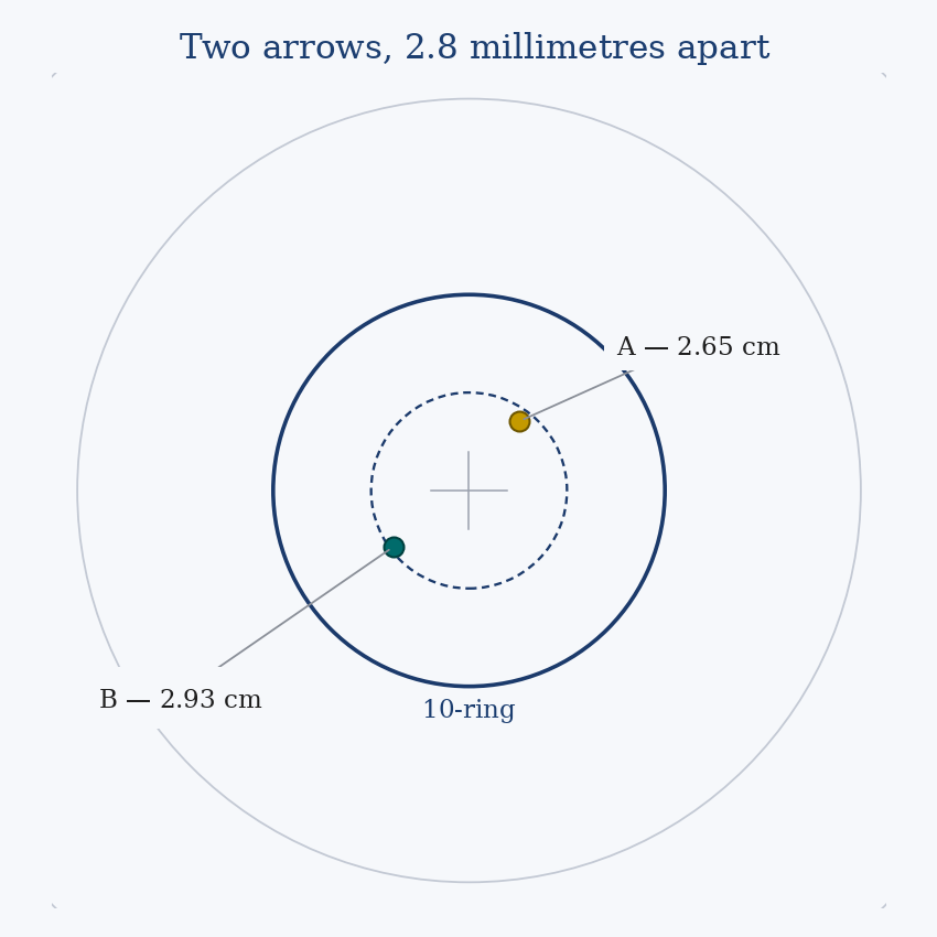
Compound uses a different match format — cumulative scoring over fifteen arrows — but ties are also resolved with a single-arrow shoot-off, so the shoot-off analysis itself applies to both bow types.
What the shoot-off is supposed to decide
Before counting how often the instrument makes an error, we have to define what counts as an error. And that definition must be fixed now, before looking at results. If “the better archer” were defined as whoever won, every rule would be infallible by construction and the question would disappear.
The criterion used here is deliberately singular: the archer with the tighter group. Nothing else. This is intentionally narrow. It excludes everything a coach would normally include in competitive skill — composure, wind management, the ability to execute the right shot when it matters — and it excludes those factors precisely when they may matter most, because no arrow carries more pressure than a shoot-off arrow.
The narrow definition has one compensating virtue: it is verifiable. Group size can be measured, compared, and tracked over time. The other qualities are real, but they do not share a single calibrated scale, and using them as the definition would mean evaluating one measurement instrument with another instrument that has not itself been calibrated.
With that definition fixed, the question becomes precise. Two archers have groups of different spreads; one is more precise than the other. Each shoots one arrow. How often does that single pair of arrows correctly reveal which archer has the tighter group?
The scale on which every answer will be read has two fixed endpoints. The floor is 50%, because that can be achieved by tossing a coin without looking at the target at all; no sensible decision rule should perform below it, since a rule wrong more than half the time could simply be inverted. The ceiling is 100%. The entire study asks where, between those two limits, one shoot-off arrow actually lies.
A refresher: the group and its spread
Only one modelling tool is needed, and readers of the set-system study already know it: an arrow group can be summarised by a single number. The reason is simpler than it sounds. An archer without a systematic directional bias misses left and right, high and low, with no privileged direction. Under that assumption, direction itself does not distinguish one archer from another; what differs is the typical distance of the arrows from centre. That characteristic distance is represented by one number, the spread of the group, denoted by the Greek letter sigma and expressed here in centimetres. Tighter group, smaller sigma, more precise archer.
The scoring rings are equally wide annuli — 6.1 centimetres each on the 122-centimetre face — and their boundaries lie at known radii. Knowing the distribution of radial distance therefore tells us how often an arrow lands in each ring. From that one spread parameter we can derive the probability of scoring ten, nine, eight, and so on with every arrow, and consequently the expected total over seventy-two arrows.
Only one equation is displayed in full in the main text, because it is the only one that needs to be visible to understand where everything else comes from: the probability that an arrow lands within a given radius of the centre as a function of spread.
F(r) = 1 − e^(−r² / 2σ²)
Read it this way: the probability of landing within radius r is zero at the exact centre and tends towards one as r becomes very large; the tighter the group, the faster the cumulative probability approaches one. A 690-level archer keeps half of all arrows within about 5.3 centimetres of centre and 90% within 9.6 centimetres; a 650-level archer requires roughly 8.4 and 15.4 centimetres, respectively, to contain the same fractions. Everything else in the analysis follows from this relationship. Readers who want the complete chain — the twenty-six steps from this equation to every published result — will find it in the appendix, with each step explained in words before symbols are introduced.
The relationship also works in reverse: every expected mean score corresponds to exactly one spread. The word expected matters. A score from one competition is one realisation among many and does not uniquely determine underlying dispersion. Whenever these pages refer to “a 690-level archer,” they mean a profile whose expected 72-arrow score is 690, not an athlete who happened to post 690 once on a scoreboard.
Fix the scale now, because it recurs throughout the study. One point in a 72-arrow total corresponds to roughly seven tenths of a millimetre of spread. An archer with an expected 690 out of 720 has a group about 4.5 centimetres wide and scores a ten roughly six times in ten; an expected 650 corresponds to a group just over seven centimetres wide and a ten roughly three times in ten. On the target, differences that look large in the results list correspond to surprisingly small changes in dispersion.
How to calculate a shoot-off that was never shot
Here is the step that is often skipped, and it is one of the most interesting parts of the problem. How can we say how often a shoot-off arrow identifies the more precise archer when that arrow was never actually shot?
The first instinct is simulation: program a computer to generate arrows, run ten million shoot-offs, and count the outcomes. That is a perfectly legitimate method and in many problems it is the only practical one. But it has a drawback: the answer contains Monte Carlo noise because ten million trials are still finite, and two runs of the same program produce slightly different estimates. When the effect being measured is only a few percentage points, that random error becomes an unnecessary complication.
No published result here is obtained that way. Every number is calculated deterministically — in closed form where possible and otherwise by numerical quadrature with a stated tolerance. A simple example shows what this means without requiring advanced mathematics.
Suppose we want the probability that A’s arrow lands closer to centre than B’s. We do not need to shoot either arrow. For every possible radial distance, we know how likely A is to land there; and for that same distance we know how likely B is to land farther out. Multiply those quantities and integrate over all possible distances. The result is the exact probability without generating any random arrows. It is conceptually the same as calculating the probability that two dice sum to a particular value: one can count the possible outcomes instead of physically rolling the dice.
For a full match the calculation becomes more elaborate but does not change in nature. An end is the sum of three arrows, so its score distribution is obtained by combining the one-arrow distribution three times through convolution, an operation that effectively enumerates every way a total can be formed. From there we derive the probabilities that A wins, ties, or loses an end. The match is then solved backward: start from terminal states where the winner is already known and work towards the beginning, set by set, calculating the probability of reaching and winning from every possible score state. It is the same general logic used to solve a simplified endgame backward from known outcomes.
A useful consequence follows. Anyone repeating the calculation tomorrow with the same method will obtain the same figures to the final decimal place. Not approximately the same — the same.
The calculation engine
A study like this produces numbers that cannot be checked by eye, so the right question is not whether they look plausible but how one would discover that they are wrong. The validation process matters because it is what earns the calculation any claim to trust.
The first level is independent double implementation. Every number in these pages was calculated twice by two programs written separately from the same mathematical specification and sharing no code. When two independent translations of the same specification produce the same result, the remaining common failure mode is misunderstanding the specification itself — precisely the risk that publishing the specification is meant to expose.
The second is random sampling used in reverse. The exact calculation does not require simulation, but simulation can still serve as an external check: a random-number generator is made to shoot a few million arrows, and the observed frequency is compared with the calculated probability, allowing for the sampling error implied by that number of trials. If the two do not agree, one of them is wrong. In this study, that check actually found an error, and in an instructive case: because of an unnoticed factor of the square root of two, the simulation was generating tighter arrows than intended. The defect appeared only in calculations that passed through the scoring rings, because comparisons between two archers are insensitive to an incorrect scale when the same incorrect scale is applied to both.
The third level concerns quantities for which there is no closed-form expression, such as elliptical groups. In those cases the calculation is numerical: the area is divided into a very large number of narrow strips and the contributions are summed. The check consists of halving the strip width and verifying that the result does not move. If it does, the grid was too coarse. Here too the check found something substantial. An early version of the formula for elliptical groups weighted directions uniformly, whereas in an elongated group the arrows are more densely concentrated along the major axis. The error reached 0.2 in probability, and it had survived a random-simulation check because that check tested the comparison between two archers rather than the calibration of each archer individually.
The fourth level is the automated test suite: sixty-seven tests included in the accompanying package, covering every published value, plus 151 reproduction checks that recalculate every numerical result in these pages one by one and stop if any value fails to match. Anyone who downloads the package can run them and inspect the outcome.
The lesson from all four levels can be reduced to one sentence: a check verifies what it knows to look for, and the two most serious errors found during this work survived checks that examined the output rather than the input on which that output depended. That is why the package is being released: so that it can be examined by someone other than the person who wrote it.
The first surprise: the rule is already as good as it can be
The instinctive objection to the shoot-off concerns how it is interpreted. Deciding a medal by looking at which of two arrows is geometrically closer to a point can seem crude, almost a disguised lottery. The mathematics says the opposite, and says it unambiguously.
The reasoning is simpler than its technical formulation suggests. Imagine looking at the two arrows on the target and having to choose between two explanations: “A is the archer with the tighter group” or “B is the archer with the tighter group.” An archer with a tighter group places arrows close to the centre more often than an archer with a wider group; an archer with a wider group places arrows farther away more often than an archer with a tighter group. If A’s arrow is closer than B’s, the first explanation accounts for what we see better than the second, because that is exactly what we would expect from a tighter shooter facing a wider one. If B’s arrow is closer, the reverse is true. There is no third case.
The calculation makes this intuition exact and also shows how strong it is. Between a 690-point archer and a 670-point archer, an arrow landing one centimetre from the centre is 68% more likely to have come from the former; an arrow twelve centimetres away is two and a half times as likely to have come from the latter. Somewhere in between—just over seven centimetres for this pair—there is a distance at which the two origins are equally likely. The important point, however, is that we do not need to know that threshold. No matter where it falls, and therefore no matter what the two spreads are, provided the groups are circular and centred, the comparison always reduces to a single question: which arrow is closer to the centre? That is why the rule can work without knowing anything about the two archers who shot.
In statistics this is a likelihood-ratio test, the standard against which a decision rule can be judged to determine whether it uses all the available information or discards some of it. The shoot-off uses all of it: neither weighting the arrows differently, nor looking at the scoring ring instead of the distance, nor any more sophisticated device can improve the decision. The rule that is often criticised is, for the task assigned to it, optimal.
One caveat must nevertheless be stated, because that optimality is not absolute. It holds under a model in which the group is circular and centred on the point of aim. If an archer had a known systematic error—a group sitting high and right, for example—the best interpretation would also use the direction of the arrow, not only its distance from the centre. No competition rule could apply such a criterion, because it would require advance knowledge of each archer’s individual bias. The accurate statement, therefore, is that the current rule is optimal given the information a judge can reasonably have, not optimal in an absolute sense.
The criticism therefore has to move elsewhere. The problem is not how that arrow is read. The problem is that there is only one of them.
How far apart would the two archers need to be?
There is a clean way to describe the value of a measuring instrument: ask how large a difference must be before the instrument can reliably detect it. A kitchen scale can distinguish 200 grams from 250 grams, not two grams from three. Applied to the shoot-off, the question becomes: how far apart must two archers be for one arrow to identify them with a given level of reliability?
The answer is a table, and the numbers in it are larger than most people would expect. Take as the reference an archer scoring 690 out of 720, roughly international-finals level.
| required reliability | required gap, in points over 72 arrows | difference in spread |
|---|---|---|
| 55 times out of 100 | 7.0 | 4.7 mm |
| 60 times out of 100 | 14.8 | 10.0 mm |
| two times out of three | 27.3 | 18.5 mm |
| three times out of four | 48.3 | 32.7 mm |
For the shoot-off arrow to identify the more precise archer even 60 times out of 100, the two archers must be separated by almost fifteen points over 72 arrows. That is a large gap: ten millimetres of spread, roughly the difference between a top-level archer and a good archer, not between two athletes similar enough to meet in a late elimination round. To reach two out of three—a level of reliability nobody would accept from a stopwatch—the gap would have to be twenty-seven points.
To put it the other way round: between two archers separated by five points over 72 arrows, corresponding to 3.4 millimetres of spread, the shoot-off identifies the better archer almost 54 times out of 100. That is information; it is not zero. But it is close to zero.
One final line from this table changes who the argument applies to. The figures above refer to international-finals level, and they become worse as performance level falls. For the shoot-off to reach 60% reliability, the required gap is 12.5 points between two 700-point archers, almost 15 points between two 690-point archers, 19 points between two 670-point archers, and almost 24 points between two 650-point archers. The lower the level, the less that single arrow can tell us. The reason is geometric: at lower levels the groups are wider, and two wide groups overlap heavily even when their scores differ substantially.
And it happens precisely between archers who are similar
At this point the picture gets worse, and not without irony. A shoot-off does not occur at random: it occurs because the two archers have reached a tie. And ties occur most often when the archers are similar. In other words, the instrument is called upon precisely in the situation in which it is least capable of telling us anything.
In statistics this phenomenon is called a selection effect. It appears whenever an instrument is judged only on cases that have themselves been filtered by the process under study. An admission test can appear weakly discriminating if it is evaluated only among applicants who ended up on the waiting list, but those candidates are, by construction, the most similar to one another. The shoot-off is in the same position.
The effect is substantial. Two identical 690-point archers finish a match at 5–5 about once in five matches; as they become more different, that probability falls, and with a twenty-point gap it is already down to about one match in ten. Combining these facts—how far apart the pairs who meet tend to be, and how often each type of pair reaches a tie—gives the quantity that actually matters: how informative the shoot-off is not in general, but in the situations in which it is truly used.
The average gap between pairs that actually reach a shoot-off lies between nine and fourteen points over 72 arrows, depending on how broad the field is. In those situations, the shoot-off identifies the more precise archer between about 55.5% and 57% of the time. The fields used for this calculation are synthetic, constructed with only two explicitly stated parameters—the mean performance level and the width of the field—and do not come from any real competition dataset.
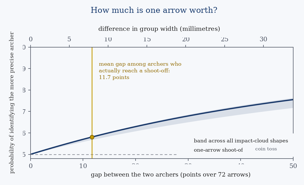
This is the first main result of the study, stated without softening: the shoot-off is close to a coin toss not because it reads the arrow badly, but because it is invoked precisely when there is almost nothing to read. Selection works against it. If shoot-offs occurred between pairs drawn at random from the field, they would identify the more precise archer between about 57% and 61% of the time, depending on field width: still little, but something. Because they occur between archers who have already reached a tie, that figure falls to just over 55%.
Why scoring and the shoot-off see the same thing differently
At this point a question arises that sounds trivial but is actually central to the problem. How can one rule be so much more informative than the other if both are observing the same archer?
The answer lies in a single curve, which is easier to understand if we first build it verbally. Take the two archers and ask, for every distance from the centre, how much more often the more precise archer lands inside that distance than the other. Very close to the centre the difference is small because neither archer gets there often; very far out the difference is again small because by then both archers are inside the radius. In between there is a hump: the region in which the tighter group is genuinely distinguishable. Call this the advantage curve.
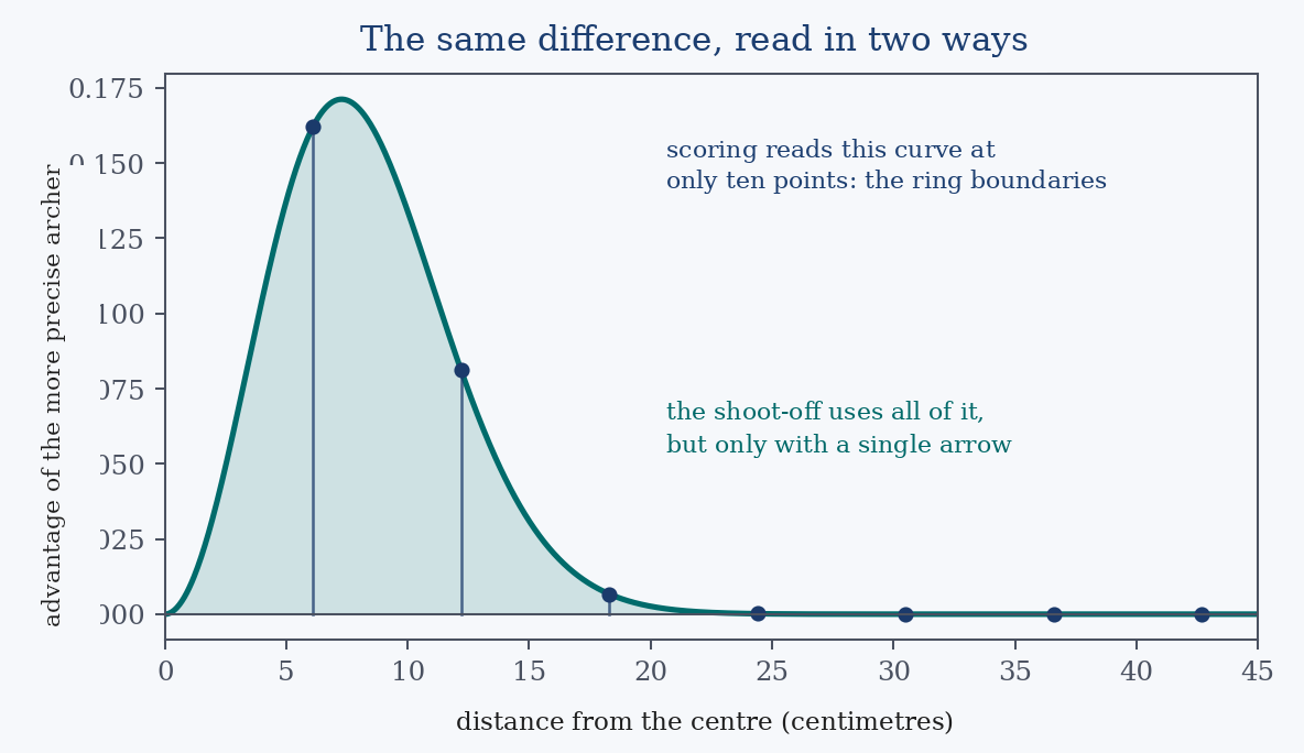
Now for the important observation, which requires an unusual but exact way of looking at scoring. The value of an arrow is the number of concentric circles within which it has landed. A ten is an arrow inside all ten circles; a seven is inside seven; a miss is inside none. Counting points and counting circles are the same operation.
A direct consequence follows. If score is a count of circles, then an archer’s mean score is the sum, across the ten circles, of the frequency with which the archer lands inside each one. For a 690-point archer that sum is 9.5833 points per arrow; multiplied by 72, it gives exactly 690—not an approximation, but an identity. The point advantage per arrow between two archers is the difference between those ten frequencies: the sum of the ten vertical differences marked in the figure; multiplied by 72, it gives the ranking-score gap. Scoring is simply this curve sampled at ten points: the scoring-ring boundaries.
The shoot-off, by contrast, does not sample ten points: it uses the entire curve, from the centre outward, without skipping any part of it. That makes the result even harsher than it first appeared, because the shoot-off is not looking at an impoverished version of the information. It is looking at the same curve, and in that sense it reads it better than the scoring system. Yet it still loses, for a reason unrelated to resolution: the score has 72 arrows with which to estimate those ten heights, while the shoot-off has one arrow with which to estimate the entire curve. The issue is not the resolution of the instrument; it is how many times the instrument is used.
There is also a useful consequence, which explains why the numerical results in this study are so stable. Because the two quantities are simply two readings of the same underlying curve, fixing the score gap also largely fixes the curve, and with it the outcome of the shoot-off. This is why, as we will see later, deforming the group in every plausible way changes the answer only slightly.
How many arrows would actually be needed?
If the limitation is sample size, the next question follows naturally: how many arrows would be required? The elegant part is that the one-arrow shoot-off is only the first rung of a ladder that can be calculated in full, and every rung represents the theoretical maximum attainable with that number of arrows. No rule, however clever, can do better.
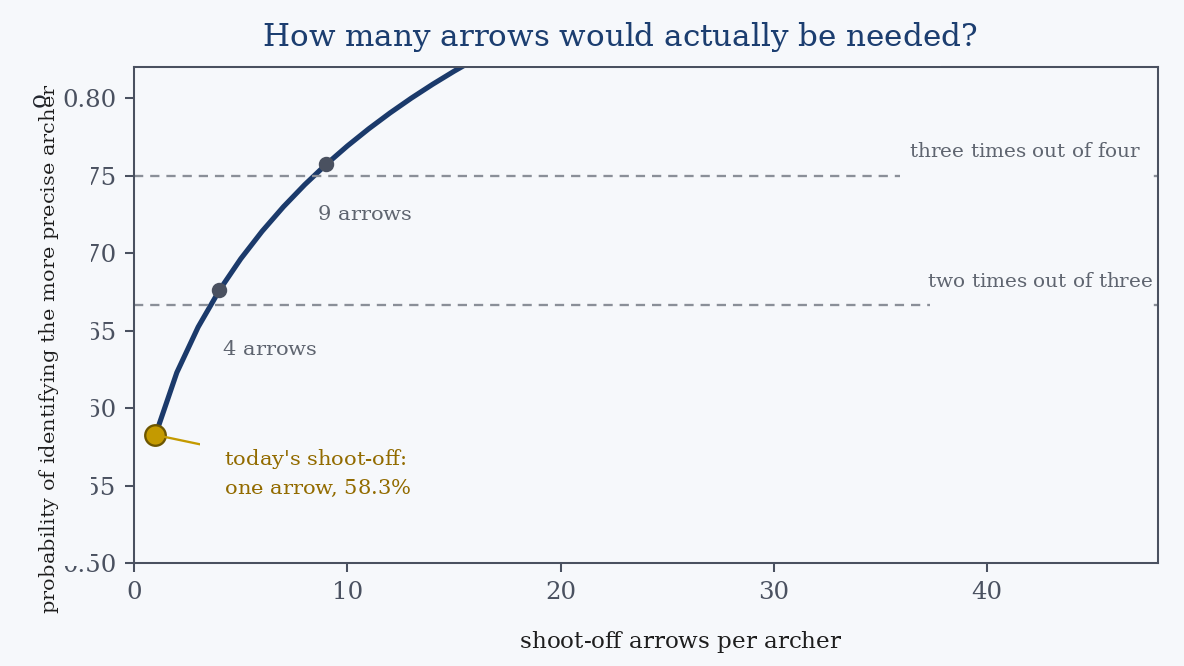
For a pair separated by twelve points, which is close to the typical gap among archers who reach a shoot-off, the ladder looks like this. One arrow: 58 times out of 100. Two arrows: 62. Three arrows—one three-arrow end: 65. In the alternating-shooting format used in finals, where each archer has twenty seconds per arrow, two additional arrows per archer mean four extra shots, a little over one minute of clock time plus administration. Reaching two times out of three requires four arrows; reaching three times out of four requires nine.
As with curves of this kind, the biggest return comes from the first step. The second and third arrows are each worth more than any arrow added later, and together they recover about two fifths of the total improvement achieved by going all the way to nine. After that the curve flattens, following the same law that governs opinion polls, laboratory measurements and any estimate obtained by repeating an observation: precision improves with the square root of the number of trials, so doubling the advantage over pure chance requires four times as many arrows. The calculation confirms this as far as it can: from one to four arrows the advantage doubles, and from four to sixteen it nearly doubles again. Beyond that the rule stops applying, not because the calculation fails but because the approximation only holds while the advantage is small; by sixteen arrows we are already approaching the ceiling. Doubling again cannot mean being right more than 100 times out of 100. At sixty-four arrows the advantage rises by only another 45%, and beyond that the gains come in tenths of a percentage point.
This is not a proposal for changing the rules; that is not the purpose of this study. It is simply the stated price list for what each additional arrow buys.
The fifteen arrows already on the target
Adding arrows costs time, and anyone producing a televised final is right to care about that cost. But there is another route that costs no shooting time at all, and it is the most interesting one: by the time two archers reach a shoot-off, they have already shot fifteen arrows each, all recorded and all on the target. Why not use those?
The idea is sound, but the pitfall is a subtle one. Those fifteen arrows have already been spent. Reaching a tie means, by definition, that the two archers have produced almost identical match profiles. Asking those same arrows to break the tie they themselves created is far less informative than it appears, and a naive calculation gives a spectacularly misleading answer.
The clearest example is the count of 10s and Xs, which was also used by the old rules and is the alternative many people would instinctively propose. If it is evaluated on the two archers without accounting for how they reached the shoot-off, it appears to identify the more precise archer 82 times out of 100: an excellent instrument. If it is evaluated on those same two archers conditional on the match having ended 5–5, its success rate falls to 56 out of 100, worse than the shoot-off it would replace. The archers and the rule are unchanged. The only difference is that the second calculation acknowledges that those arrows have already produced a tie.
Putting numbers on the filter makes its strength obvious. For the reference pair, without conditioning, the number of 10s scored across the fifteen arrows differs by an average of three and is equal only about once in ten cases. Among matches that specifically end 5–5, the average difference falls to one and the counts are equal in almost one case out of three. Counting 10s is not intrinsically a poor criterion. It simply has almost nothing left to say by that stage of the match, because whatever information it contained has already been expressed through the five sets.
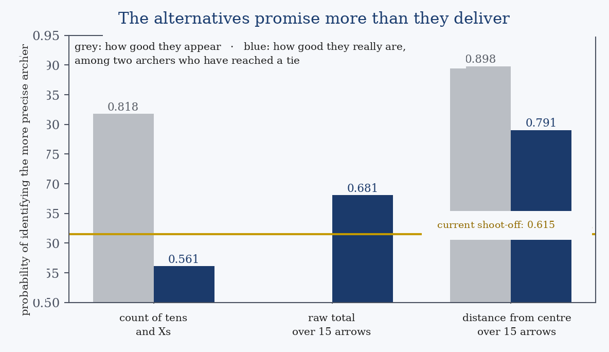
Only one option survives, and it uses information the match already possesses but does not currently exploit. The rule is precise: sum the squared distances from the centre for all fifteen arrows, and the smaller total wins. The square matters. The model identifies squared distance, not simple distance, as the optimal way to read all fifteen arrows, for the same reason that with one arrow the optimal reading is simply whichever arrow is closer to the centre.
It works because scoring censors information. Two archers with exactly the same ring-score profile have exhausted all the information contained in those scores, but not the information contained in where each arrow landed within its ring. A 10 on the line and a 10 one centimetre from the centre are worth the same number of points, but they are not the same shot. Measuring how far each of the fifteen match arrows landed from the centre raises the success rate, for a pair separated by eighteen points, to 79 times out of 100 compared with 62 for the shoot-off. For the tighter twelve-point pair, which is the more typical case, it rises to 72 compared with 58. Depending on the pair, the gain remains between fourteen and eighteen percentage points.
This is the most concrete conclusion in the entire study. In international finals where optical scoring systems have been used, the position of each arrow has been recorded and the competition rule has discarded that information. The point needs to be stated precisely, however: the rules require electronic scoring, not the recording of impact coordinates. Feasibility is demonstrated by systems that have already been used in competition; it is not an inherent property of every electronically scored target.
The bracket: where it matters most, it knows least
So far we have looked at one match at a time. An Olympic competition, however, is a bracket: sixty-four archers, sixty-three matches, and six consecutive wins to take gold. Combining the mechanics of the bracket with the mechanics of the shoot-off produces a picture that neither component reveals on its own.
The composition of the field has to be stated because the result depends on how those sixty-four archers are distributed. In the reference field used here, the top seed is four points ahead of the second seed, and scores then decline across the bracket over a forty-point range. The bands shown below span twelve fields with different shapes and ranges. In a typical bracket, the set system sends between eight and ten of the sixty-three matches to a shoot-off, a little less than twice as many as cumulative scoring would. But the important point is not the total number. It is where those shoot-offs occur.
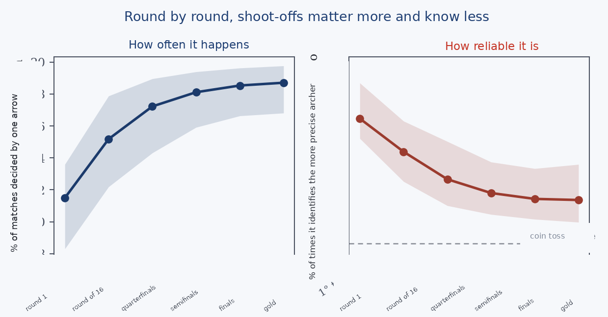
In the first round, just over one match in ten reaches a shoot-off, and there the shoot-off identifies the more precise archer between 57% and 61% of the time. In the gold-medal match, just under one match in five reaches a shoot-off, and there it identifies the more precise archer only between 51.5% and 55.5% of the time. The two curves move in opposite directions for the same reason: the bracket acts as a filter, progressively removing weaker archers so that those who reach the later rounds are increasingly similar. The mean gap between opponents falls from about fifteen points in the first round to about five in the final.
In practical terms, the model says that roughly one gold-medal match in five is decided by a single arrow, and that arrow identifies the more precise archer only a little more than 53 times out of 100. It is about the worst possible combination of importance and reliability, and it is not an unlucky accident: it is a structural consequence of a single-elimination bracket.
How much the result depends on the assumptions: the group shapes tested
A sceptical reader has a legitimate objection at this point. The framework assumes a circular group centred exactly on the point of aim, whereas real groups are often elliptical, may be off-centre, and occasionally contain a shot that bears little resemblance to the rest. Worse still, a score constrains the group at the scoring-ring boundaries but says very little about how arrows are distributed within the 10-ring, which is precisely where many shoot-offs are decided.
That objection is valid, which is why this study does not merely estimate a single answer: it bounds the answer. Instead of choosing one group shape and trusting it, the calculation is repeated across a family of plausible shapes—ellipses up to three times longer than they are wide, centres displaced by a full spread, groups capable of producing extreme outliers, and very tight cores with broad tails—and the result is reported as a range rather than a single point.
One of these shapes describes an archer anyone who has spent time on a shooting line will recognise. The Gaussian bell curve is extremely unforgiving of large errors: for a 690-point archer it predicts an arrow worse than a 7 only about once every three million shots, effectively never in an archery career. Other groups can have the same typical spread while producing those disasters much more often. In statistical language they have heavy tails. Under one such model, the same kind of arrow occurs about once every 170 shots, roughly once every two and a half competitions. It is the archer who shoots exceptionally well for seventy arrows and then throws one away for no obvious reason.
The interesting part is that, because this archer must still average 690 points, the model has to compensate elsewhere: the core of the group becomes tighter. Such an archer puts 67% of arrows in the 10 compared with 61% under the Gaussian model, and 29% in the X compared with 21%. This archer is neither better nor worse; the distribution is simply shaped differently. That is exactly the kind of difference a robustness analysis ought to absorb.
There is an easy mistake to make in running such a test. Changing the shape of the group is only half the job. Immediately afterwards, the group must be recalibrated back to the original expected score by tightening or widening it as necessary. If that step is skipped, the resulting archer is not merely different but also weaker, and an effect caused by lower performance is incorrectly attributed to group shape.
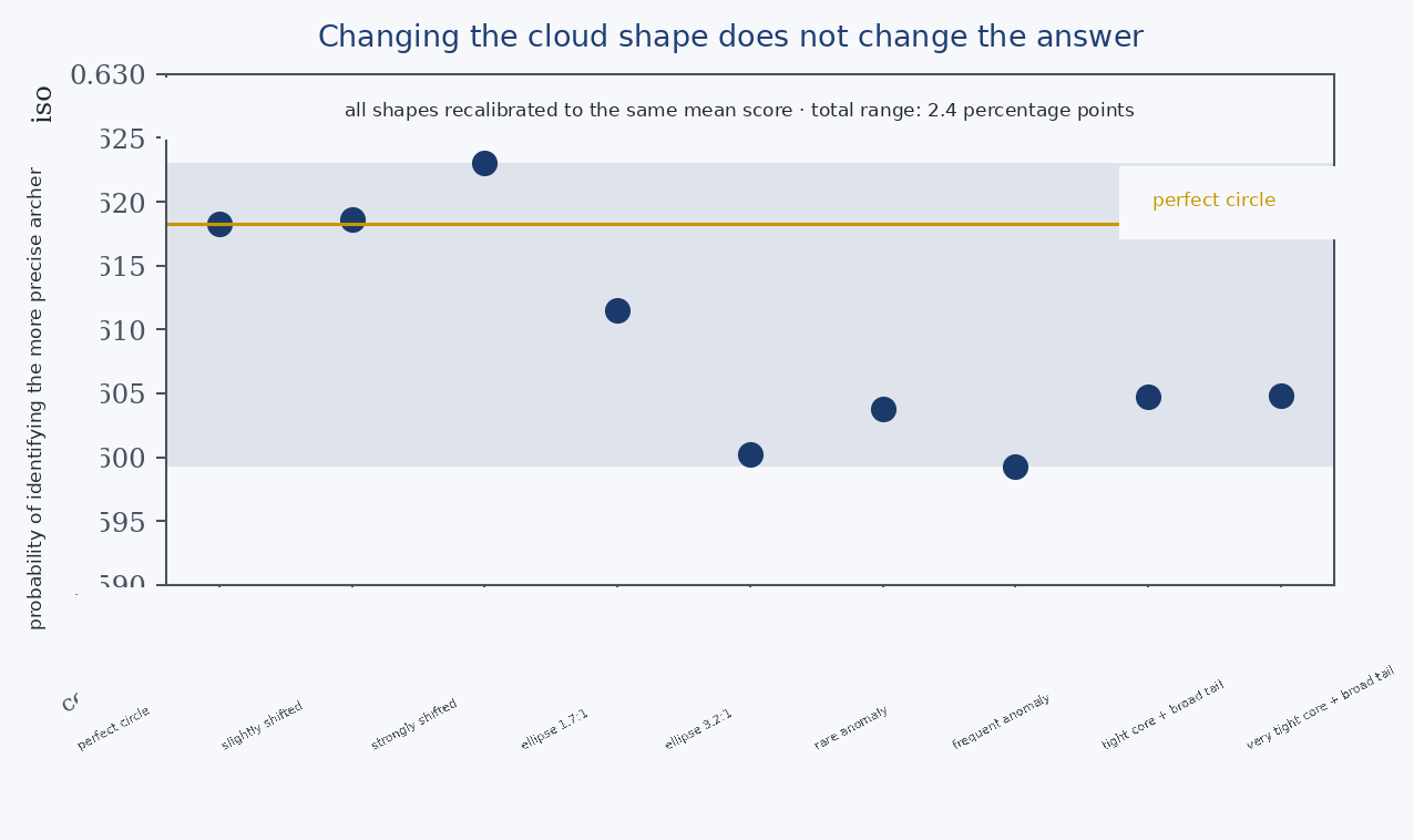
The result is that shape matters surprisingly little. From a perfect circle to an ellipse three times longer than it is wide, through displaced centres and heavy-tailed distributions, the answer moves by only 2.4 percentage points in total. That variation should not be hidden, because relative to the total advantage over chance it is not negligible. But none of the tested shapes makes the shoot-off even remotely reliable, and none reduces it to pure chance. Across every family tested, it remains what it is: a weak instrument.
We have already seen why the result is so stable. Score and shoot-off are two readings of the same advantage curve, and fixing the point gap strongly constrains that curve. This is not luck; it is a consequence of the structure of the problem.
There is also a route that cannot be taken. One might ask whether the entire model could be avoided by using public competition data and simply counting how many arrows land in each scoring ring. It cannot, and the calculation shows exactly why: ring counts alone leave the answer unidentified within a range 43 percentage points wide, which is useless, and subdividing the centre into progressively finer circles does not close that range. Bounding the answer through a model family is not a matter of convenience. It is the only route available from the information we have.
What the model does not see
Now comes the part that matters most: everything the model deliberately ignores. In the model, every shot is generated independently from the same unchanging group. There is no rising tension, no fatigue accumulating in the arm, no end in which everything suddenly falls apart. Here the limitation matters more than elsewhere, because a shoot-off arrow is not just another arrow. It is arguably the highest-pressure shot in the sport, taken with the knowledge that nothing follows it.
Treating it as if it were distributed like the preceding fifteen arrows is a strong assumption, and there is evidence that it is false. Analyses comparing shoot-off arrows with match arrows in real competitions have reported a performance drop specifically in the shoot-off, and the effect grew larger in the most consequential competitions, though only among the women in that study. Subsequent work points to substantial individual and contextual heterogeneity. The existence of some performance decrement has empirical support; its magnitude, causes and population distribution remain open questions, and the calculations in these pages do not resolve them. Knowing that such an effect exists is nevertheless enough to guide how the rest of the results should be interpreted.
The direction of the bias depends on how pressure acts, and the mathematics is instructive. If pressure widened both archers’ groups proportionally—say by 20% for each—nothing would change at all, because shoot-off discrimination depends only on the ratio between the two spreads, not on their absolute size. If pressure adds an archer-specific error component to each distribution, which is arguably more natural, then the two groups become more similar than the archers themselves and the shoot-off becomes even less informative than estimated here. If, on the other hand, there is a genuinely distinct performance trait—composure, for example, or execution under pressure—then the shoot-off may be measuring that trait, and may be measuring something different from precision quite well. In that case it would not be an imprecise instrument but an instrument pointed at a different construct. The present model cannot distinguish those possibilities, and anyone asserting the second interpretation carries the burden of measuring it.
We can, however, do more than merely state the limitation: we can quantify it. If pressure adds an error component to both archers, that component can be introduced into the model and its effect on the answer measured. An intuitive currency makes the size of the effect easier to grasp. Suppose the shoot-off arrow under pressure behaves as if it were shot by an archer a certain number of qualification points weaker. A ten-point decrement means that the better archer, at the moment of the shoot-off, behaves like a 680-point archer rather than a 690-point archer.
The result is more robust than might be expected. For the typical pair separated by twelve points, the no-pressure shoot-off identifies the more precise archer 58.3 times out of 100. With a ten-point decrement, that falls to 56.5; with twenty points, to 55.2; with thirty, to 54.3. A thirty-point decrement is enormous and, within the model, separates archers of clearly different performance levels. Yet it costs only four percentage points of an initial advantage over chance of just over eight.
The inverse calculation makes the point even more clearly. To push shoot-off success down to 55 out of 100 would require a decrement of about twenty-two points; reaching 52 would require seventy-eight; and reducing it to essentially a true coin toss, 51 out of 100, would require roughly 140 points. A 140-point decrement would mean a 690-point archer performing, for that moment, like a 550-point archer. Within this model, that is not a remotely plausible order of magnitude.
The same is true of the two headline figures. The weighted probability—the figure a little above 55 out of 100—falls to 54.6 with a ten-point decrement and to 53.8 with twenty. The gold-medal final falls from 53.5 to 52.7 and then to 52.1. Pressure erodes the signal; it does not reverse the story.
Two separate conclusions follow, and they should be kept distinct. First, the stated limitation is real and pushes in the unfavourable direction: accounting for it makes the shoot-off less informative, not more. Second, it does not make the shoot-off sufficiently less informative to change the overall conclusion. Eliminating its discriminative power would require performance collapses of an implausible order of magnitude. The study’s result therefore does not hang entirely on the independence assumption. It survives the violations calculated here, namely scenarios in which pressure affects both archers in the same way: in those cases discriminative power either remains unchanged or decreases; it never increases. If the two archers respond differently to pressure, however, the direction of the effect is not determined by this model and would have to be established empirically.
One case remains outside the calculation and should be stated explicitly. If pressure did not affect the two archers in the same way—if one coped with it and the other did not—the effect could run in either direction and might even increase the shoot-off’s discriminative power, in which case the shoot-off would be measuring pressure resilience rather than precision. This is the same possibility raised above, and the answer is the same: the model neither excludes nor demonstrates it. Anyone making that claim has the burden of measuring it.
Limitations
Three further limitations need to be stated, because they define what these pages can and cannot support.
First, ability is represented here by a single quantity: spread. That simplification is declared in advance. An archer is also defined by endurance across a long competition, wind management, the ability to recover from a poor end, and many other qualities. None of those enters these calculations.
Second, the comparison between rules changes the arithmetic, not athlete behaviour. Under a different shoot-off rule, archers would probably shoot differently—perhaps from the very first set—whereas the counterfactual calculation leaves the arrows where they are and changes only how they are interpreted. This is a common limitation of counterfactual analyses of sporting rules and must be kept in mind whenever a result is phrased as “would have happened.”
Third, and most subtly, “who was really the stronger archer” in a particular match is not observable from that match alone. With many competitions and an explicit model, one can estimate which archer has the tighter underlying group and quantify the uncertainty around that estimate. What one can never obtain is certainty about that single day, because the question remains counterfactual.
The study should therefore be read for what it is: a modelling study. It describes the behaviour of the decision instrument in the abstract and does not claim to say what that instrument recorded in any specific real-world match. A study measuring the actual margins in completed shoot-offs—how many millimetres truly separated the two arrows—would be a different study, would require impact-coordinate data recorded by electronic target systems, and remains to be done.
What to take away
For the archer. Losing a shoot-off is not a verdict on your ability, and that statement should be taken literally. In the situations in which shoot-offs actually occur, the deciding arrow identifies the more precise archer only a little more than 55 times out of 100, and in a final about 53. This means that against an opponent at a very similar level, losing a shoot-off occurs almost half the time even when you are the archer with the tighter underlying group. Practising the shoot-off shot makes sense for many reasons, but a single outcome is not enough to support a technical diagnosis. It is one clue to place alongside video, subjective feedback and performance history, not a conclusion in itself.
For the coach. A shoot-off is the smallest possible sample in this sport and should be treated accordingly: one arrow. No training plan should change solely because of a shoot-off result, in either direction, although the arrow may still be informative when considered with other evidence. The order of magnitude is this: for that one arrow to become 60% reliable, the gap has to be almost fifteen points over 72 arrows. That alone makes clear how little can safely be inferred from a single shot.
For rule-makers. The limitation is not the decision rule itself, which is already the best possible reading of that arrow, but the sample size. The two main remedies have very different costs and are best compared on the same twelve-point reference pair, the typical case. Adding two arrows per archer costs a little over one minute of alternating shooting, plus administration time, and raises reliability from 58 to 65 out of 100. Reading the distance from the centre of the fifteen arrows already shot costs no additional shooting time and raises it to 72, but it is not free: it requires targets capable of recording coordinates with sufficient accuracy, together with calibration, verification and appeal procedures, plus a fallback rule for system failure. That is a regulatory and technological cost rather than a time cost, and it should be counted as such.
One arrow, in the wrong place
The picture that emerges is restrained and slightly uncomfortable. The shoot-off is not a lottery: it carries information, and it extracts that information as efficiently as possible under its assumptions. But those assumptions amount to asking one arrow to arbitrate between two people similar enough to have reached a tie, and under those conditions the best possible reading of a single arrow is worth only a little more than a coin toss.
What matters most is not even the number, but where it appears. A weak instrument can be acceptable when used for low-stakes decisions; here the opposite happens by construction. As the bracket advances, shoot-offs become more frequent and less reliable, until in the gold-medal final a single arrow decides almost one match in five while distinguishing the two opponents only about 53 times out of 100.
There is, however, a more useful way to interpret all this, and it is not an accusation against the rules. A shoot-off does not claim to measure; it claims to conclude. Its purpose is to put a full stop where the competition format has run out of room, in front of an audience and within a schedule. It performs that task exceptionally well: it is fast, easy to understand and visually decisive. The misunderstanding begins when closure is mistaken for measurement, and a hierarchy is read into an arrow that cannot establish one.
Keeping those two functions separate takes nothing away from the sport and removes a great deal of unnecessary bitterness. The loser of a shoot-off has lost something close to a coin toss, not a comprehensive technical comparison; if that athlete was the more precise archer, the odds were, if anything, slightly in their favour. The winner has legitimately won the match, not proved an argument about superior underlying precision. Those two statements coexist without contradiction. The mathematics is useful precisely because it keeps them separate.
One final observation makes the problem tractable rather than tragic. The shoot-off’s weakness does not arise from anything mysterious; it arises from asking a single observation to settle what fifteen observations had failed to settle. The two possible remedies ultimately do the same thing: they move the decision from one observation to many. Additional arrows do so by creating new observations; fine-grained coordinate analysis does so by recovering information from the fifteen arrows already shot that rounded ring scores had discarded. No new theory is required. The decision simply has to stop resting on one arrow alone.
Note on data, sources and method
No data from real individuals enter these pages, nor would such data be required for the calculations presented here. There are no scores from identifiable archers, no reconstructed real competitions, no names and no rebuilt rankings. Everything comes from three public and impersonal sources: target dimensions established by the rules; the competition rules governing the two scoring formats and the shoot-off; and a statistical model of how arrows are distributed around the point of aim.
The recurring scores—690, 688, 678—belong to nobody. They simply place the reasoning at realistic performance levels, much as a mechanics problem might posit a one-kilogram body. The particular body does not exist; the scale does.
No result here is generated by Monte Carlo simulation. Quantities are obtained in closed form where possible and elsewhere by deterministic numerical quadrature, with a stated tolerance checked for convergence. Deterministic does not mean exact: numerical quadrature has discretisation error, however carefully controlled. It means that someone repeating the calculation tomorrow will obtain the same figures without sampling variability. Where no closed form exists, as for elliptical groups or mixture distributions, the model integrates numerically on a deterministic grid, states the grid step and verifies that halving it does not materially change the result. The single-match results—the arrow-count ladder, distinguishability thresholds, the collapse of the no-extra-arrow alternatives and the group-shape family—were recalculated by a second independent implementation written separately from the same mathematical specification and checked against random sampling used solely as an external validation, never as the source of the estimates. The bracket-level figures were also replicated by that second implementation using an independent tournament module and reproduced across four field shapes. They are nevertheless reported as bands because they depend on field composition rather than on a single scenario.
The competition rules described here—the set format, cumulative scoring, one-arrow shoot-off and shooting times—are those in the current World Archery rules. The only result not produced within this study is the shoot-off performance decrement mentioned among the limitations. That result comes from previously published analysis of competition data, is cited only to guide interpretation, and enters none of the calculations in these pages.
The accompanying package contains the code, mathematical specification and tests. It is designed so that a reader can reproduce every calculation, disprove it, or apply it elsewhere. Error reports are welcome; contact details are provided on the website.
Mathematical appendix
The main essay displays only one formula: the formula translating spread into the probability of landing within a given distance of the centre. That is deliberate. It is the only equation a reader needs to see in order to understand where everything else comes from.
This appendix contains the twenty-six formulas evaluated by the engine to produce every number printed in the preceding pages. It provides the complete mathematical translation, with enough context for a reader who is not a professional mathematician to understand what each expression says, why it has that form and what it cannot tell us. Readers interested only in reproduction can skip the prose and use the equations; readers interested in understanding how a measurement problem of this kind works may find that the prose is the more useful part.
Structure of each entry
Each formula has at least four parts. “In words” states what is being calculated without symbols. “Formula” displays it. “Where it comes from” reconstructs the derivation, usually in two or three lines. “A numerical example” applies it to a concrete case, most often the 690-point archer or the recurring 688-versus-670 pair, so that every formula has at least one verifiable value. Where necessary, a final line states what the formula does not cover: the conditions beyond which it no longer applies.
Notation and units
The study moves between three units of measurement, and confusing them is the quickest way to obtain absurd numbers. Target geometry is expressed in centimetres on the target plane. The calculation engine works in milliradians—angular units—so that the formulas apply at any shooting distance. The essay speaks in centimetres because that is how an archer naturally sees a group. The bridge between them is simple: at seventy metres, one milliradian subtends seven centimetres.
One term could be ambiguous, but is used here in only one sense. “Spread” always means the standard deviation of an individual archer’s group. When referring to how widely the sixty-four competitors’ expected scores are distributed across a bracket, the term “field range” is used instead.
| symbol | meaning |
|---|---|
| σ | spread: the standard deviation of the impact points along each axis. It is neither the group radius nor its diameter. |
| r, ρ | distance from the centre. r in centimetres, ρ in milliradians. |
| r, ρ | distance from the centre of a single arrow already shot; F(r) is its cumulative distribution function. |
| w | width of one scoring ring: 6.1 cm on the 122 cm face. |
| rₓ | radius of the X ring: 3.05 cm, half the width of one scoring ring. |
| k | scoring-ring index, from 1 (the 10-ring) to 10 (the outermost scoring ring). |
| D | shooting distance, always 70 m in these pages. |
| F(r) | probability that an arrow lands within radius r. |
| pᵥ | probability that a single arrow scores exactly v points. |
| μ | expected score per arrow; the 72-arrow total is 72μ. |
| r, ρ | advantage function: how much more often the more precise archer lands within radius r. |
| pₛₒ | probability that the shoot-off identifies the more precise archer. |
| c | ratio of the squared spreads, σᵇ²/σᵃ². |
| S | score of a three-arrow end. |
| π₅₅ | probability that a set-system match ends 5–5. |
| θ, g(θ) | angle around the centre and angular weighting of the elliptical group (S21). |
| ν | parameter controlling tail thickness (S23): high = Gaussian-like; low = heavy-tailed. |
| j, u | seed index in the bracket and field-profile variable (S25). |
| Iₓ(a,b) | regularised incomplete beta function. |
The formulas are meant to be read in order because each one uses only preceding formulas; none depends on one that appears later. Some entries refer forward, but only in statements describing limitations or explaining why a quantity matters: to point to where a special case is handled, never to use that later result in the derivation.
| group | contents |
|---|---|
| S01–S05 | Target geometry and the group model: converting centimetres to angles, describing the shape of dispersion, and deriving the probability of each score. |
| S06–S08 | The bridge between spread and score in both directions, and the advantage function that connects them. |
| S09–S13 | The shoot-off: the rule, its probability of identifying the more precise archer, the proof of optimality, the distinguishability threshold and the arrow-count ladder. |
| S14–S19 | The match and conditioning: three-arrow ends, sets, backward induction, the probability of a 5–5 tie, and rules that reuse arrows already shot. |
| S20–S26 | Robustness and tournaments: recalibration, elliptical groups, displaced centres, heavy tails, parametric fields, propagation through the bracket and a negative control. |
Part I — The target and the group
Five formulas are enough to specify two things: the geometry of the target and the mathematical description of an arrow group.
S01 · Target-face geometry
In words. The 70-metre target is a disc 122 cm in diameter, divided into ten concentric scoring rings of equal width. That uniformity makes everything that follows simpler: the ring boundaries are not a list of unrelated numbers but multiples of a single quantity.
rₖ = w · k , k = 1,…,10 vₖ = 11 − k w = 6.1 cm rₓ = 3.05 cm
Where it comes from. The outer radius of ring k is k times the ring width w. The score assigned to that ring is 11 minus k: the first ring scores ten points, the second nine, and so on down to the tenth, which scores one. At the centre is an additional circle of radius 3.05 cm, exactly half a ring width, called the X ring. It still scores ten points and is used in other contexts to resolve ties.
A numerical example. The 10-ring has radius 6.1 cm; the 9-ring extends to 12.2 cm; the outer edge of the target is 61 cm from the centre. A top-level archer has a spread of roughly three quarters of a single scoring-ring width.
S02 · Angular scale
In words. An arrow group does not have a meaningful absolute size; it has an angular size. The same aiming error produces a group twice as wide at twice the distance. Working in angles rather than centimetres allows the same formulas to apply at any distance.
ρ = r / D at 70 m: 1 mrad = 7 cm
Where it comes from. A milliradian is one thousandth of a radian, and for small angles one radian subtends a length equal to the distance D. Therefore, at a distance of D metres, one milliradian subtends D millimetres: at seventy metres, seventy millimetres, or seven centimetres.
A numerical example. A 6.1 cm ring width subtends 0.871 mrad at seventy metres. The spread of a 690-point archer is 4.4613 cm, or 0.637 mrad.
S03 · The group
In words. For an archer without systematic bias, impacts are modelled around the point of aim as a two-dimensional Gaussian distribution: dense near the centre, progressively sparser farther away, and equally distributed in every direction.
(x, y) ~ N(0, σ² I)
Where it comes from. This is the standard model for measurement error and follows from treating the final error as the sum of many small, approximately independent causes—aiming, release, wind, arrow behaviour and so on. Circular symmetry adds the assumption that no direction is privileged, which is reasonable for a well-tuned archer but not for one with a known directional bias.
What it does not cover. Elliptical groups, displaced centres and grossly misplaced shots. These cases are treated in S21, S22 and S23, and the essay’s conclusions are tested there as well.
S04 · Distance from the centre
In words. The score depends not on the Cartesian position of the arrow but only on its distance from the centre. We therefore need the probability that this distance is less than a given radius.
F(r) = P(R ≤ r) = 1 − e^(−r² / 2σ²)
Where it comes from. If the two components of the error are independent normal variables with the same standard deviation, distance from the centre follows a Rayleigh distribution. Integrating the two-dimensional Gaussian over a disc of radius r gives the closed form above, made possible by circular symmetry.
A numerical example. For the 690-point archer, whose spread is 4.4613 cm, the probability of landing inside the 10-ring is F(6.1) = 0.607; inside the X ring it is F(3.05) = 0.208.
S05 · Probability of each arrow score
In words. An arrow scores k points when it lands between the inner and outer boundaries of the corresponding scoring ring. The probability of that score is therefore the difference between two cumulative probabilities from S04.
pₖ = F(r₁₁₋ₖ) − F(r₁₀₋ₖ) , k = 1,…,10 p₀ = 1 − F(r₁₀)
Where it comes from. This is simply the definition of an annulus: the probability of landing within a scoring ring is the probability of landing inside its outer boundary minus the probability of landing inside its inner boundary. A score of zero collects everything outside the scoring face.
A numerical example. For a 690-point archer, the 10 occurs on 60.7% of arrows, the 9 on 36.9%, the 8 on 2.4%, and anything below 8 is essentially absent—about two arrows in ten thousand. The eleven probabilities sum to one by construction, which is the first check performed by the calculation engine.
Part II — From score to spread, and back again
Three formulas build a two-way bridge between what appears on the scoreboard and what happens on the target. The third is one of the study’s main theoretical contributions.
S06 · Expected score as a count of circles
In words. Mean score per arrow can be written in two equivalent ways. The obvious one multiplies each possible score by its probability and sums the results. The less obvious, but much more useful, expression sums the ten probabilities of landing inside each scoring-ring boundary.
μ = Σₖ k · pₖ = Σₖ₌₁¹⁰ F(rₖ)
Where it comes from. An arrow’s score is the number of concentric scoring circles within which it lies: a 10 lies inside all ten circles; a 7 lies inside seven. Counting points and counting circles are the same operation, and reversing the order of summation converts the first expression into the second.
A numerical example. For a 690-point archer, the second sum is 9.5833 points per arrow. Multiplied by 72, that is exactly 690 points. It is not an approximation but an identity, and the engine verifies it on every run.
S07 · Inversion
In words. The relationship between spread and expected score is monotonic: a tighter group always implies a higher expected score. The relationship can therefore be inverted, assigning a unique spread to each expected mean score.
σ(T) : 72 · μ(σ) = T , unique solution
Where it comes from. The function mapping σ to μ is continuous and strictly decreasing because widening the group lowers the probability of landing inside every scoring-ring boundary. A function with those properties has a unique inverse, found numerically here by bisection.
A numerical example. An expected 72-arrow total of 700 corresponds to a spread of 3.7817 cm; 690 to 4.4613 cm; 680 to 5.1375 cm; 670 to 5.8135 cm; and 650 to 7.1654 cm. Around 690, the local slope is about 0.68 millimetres per point. That is the conversion factor repeatedly used throughout the essay.
What it does not cover. A score from one competition is one realisation among many, not the expected score itself. The inversion links spread to the long-run mean, not to a single observed total.
S08 · The advantage function and the structural identity
In words. Given two archers, consider at every distance from the centre how much more often the more precise archer lands inside that radius. The resulting curve is zero at the centre, returns towards zero far away, and has a hump in between. That single curve determines both the expected score gap and the outcome probability of the shoot-off.
Δ(r) = Fᴀ(r) − Fᴮ(r) Δμ = Σₖ₌₁¹⁰ Δ(rₖ) pₛₒ = ½ + ∫ Δ(r) dFᴀ(r)
Where it comes from. The first identity follows from applying S06 to each archer and subtracting. The second is obtained by expressing the probability that A’s arrow is closer as an integral and adding and subtracting one half. The important point is that both quantities are functionals of the same curve: the scoring system samples it at ten points, while the shoot-off integrates across the full curve.
A numerical example. For the 688-versus-670 pair, the curve reaches its maximum 7.3 cm from the centre; the sum of the ten sampled heights is 0.2500 points per arrow, equivalent to 18.0 points over 72 arrows; and the integral gives a shoot-off probability of 0.6153. The two numerical routes converge to the same result, and the residual integration error halves when the grid step is halved—the appropriate convergence check for numerical quadrature.
Why it matters. This is why the study’s results are so insensitive to group shape: once the score gap is fixed, the advantage curve is strongly constrained, and so is its integral.
Part III — The shoot-off
Five formulas describe the rule, its value, why it is the best possible reading of the available information, how far apart two archers must be for it to work reliably, and what changes when more arrows are added.
S09 · The rule
In words. Each archer shoots one arrow; the arrow closer to the centre wins. If the judge cannot determine which is closer, the process is repeated.
A wins ⇔ Rᴀ < Rᴮ
Where it comes from. This is the competition rule, not a modelling assumption. The historical wording—first compare the scoring ring, then the distance—always produces the same winner, because the rings are concentric circles and an arrow that is closer to the centre cannot lie in a lower-valued ring than a farther arrow. The two formulations are equivalent.
What it does not cover. The case in which both arrows miss the scoring area, and the case in which measurement cannot resolve which arrow is closer. Both trigger another shoot-off under the rules. The continuous model does not represent exact ties because they have probability zero.
S10 · How often it identifies the more precise archer
In words. The probability that the tighter-group archer wins depends only on the ratio of the two spreads and has a surprisingly simple form.
pₛₒ = P(Rᴀ < Rᴮ) = σᴮ² / (σᴀ² + σᴮ²)
Where it comes from. For a circular Gaussian group, squared distance from the centre follows an exponential distribution whose rate is the reciprocal of twice the variance. The probability that one independent exponential variable is smaller than another is a ratio of their rates; rearranging gives the formula above.
A numerical example. The probability that the shoot-off identifies the more precise archer is 0.5365 for a 690-versus-685 pair; 0.5701 for 690 versus 680; 0.6153 for 688 versus 670; and 0.7821 for 700 versus 650. These are probabilities: 0.6153 means a little over 61 times out of 100.
Why it matters. The formula is scale-invariant: multiplying both spreads by the same factor leaves it unchanged. That is why pressure that proportionally widened both groups would leave discriminative power unchanged.
S11 · Why closest to the centre is the optimal rule
In words. Among all decision rules that could be constructed from the two arrows, none performs better than the current one. Applying it does not require knowing the spreads; it requires only knowing which observed distance is smaller.
log Lᴀ − log Lᴮ = (Rᴮ² − Rᴀ²) · ( 1/2σᴀ² − 1/2σᴮ² )
Where it comes from. Compare two hypotheses—“A is the tighter archer” against “B is the tighter archer”—by writing the likelihood of the observed data under each and taking their ratio. The second factor is positive exactly when σᴀ is smaller than σᴮ, so the sign of the entire expression depends only on the first factor: which arrow is closer. The Neyman–Pearson result establishes the likelihood-ratio test as the most powerful test for this simple-vs-simple comparison.
A numerical example. Between a 690-point archer and a 670-point archer, an arrow one centimetre from the centre is 68% more likely to have come from the former; at twelve centimetres it is two and a half times as likely to have come from the latter, and just beyond twelve and a half centimetres exactly three times as likely. The indifference threshold is 7.2 cm. Crucially, the rule does not need to know that threshold.
A comparison. If the rules used only the scoring ring—higher ring score wins, with a random decision when both arrows are in the same ring—the same 688-versus-670 pair would yield 0.5955 instead of 0.6153. Almost two percentage points are lost by discarding the exact position of the arrow within the ring. That difference measures the value of the fine-grained comparison already used by the current rule.
What it does not cover. Optimality holds under the model in S03. With a known systematic directional bias, the optimal decision would also use the arrow’s direction. No practical competition rule could apply such an athlete-specific criterion, so the correct statement is that the current rule is optimal given the information a judge can reasonably possess.
S12 · Minimum discriminable difference
In words. Inverting S10 gives the performance gap required for the shoot-off to distinguish two archers with a specified reliability. This is the standard way to state the resolution of a measurement instrument.
pₛₒ = p ⇒ c = p/(1−p) , σᴮ = σᴀ√c , ΔT = 72·μ(σᴀ) − 72·μ(σᴮ)
Where it comes from. Set the S10 expression equal to the desired probability, solve for the ratio of spreads, and convert that ratio into qualification points using S07. The three currencies—millimetres, points over 72 arrows and a dimensionless variance ratio—are simply three ways of expressing the same difference.
A numerical example for two archers around the 690 level: 55% reliability requires a 7.0-point gap, corresponding to 4.7 mm difference in spread; 60% requires 14.8 points and 10.0 mm; two times out of three requires 27.3 points and 18.5 mm; three times out of four requires 48.3 points and 32.7 mm.
The threshold depends on performance level and becomes less favourable as level falls. Reaching 60% requires a 12.5-point gap between two 700-point archers, 14.8 points between two 690-point archers, 19.3 points between two 670-point archers and 23.8 points between two 650-point archers, always on the 72-arrow scale. The reason is geometric: wider groups overlap heavily even when the expected-score gap is held constant.
S13 · The arrow-count ladder
In words. If n arrows rather than one were shot, the probability of identifying the more precise archer would increase according to an exact expression, and that value is the theoretical maximum attainable by any decision rule using n arrows.
P(n) = I₍ᶜᐟ₍₁₊ᶜ₎₎(n, n) , c = σᴮ²/σᴀ²
Where it comes from. The sum of squared distances from the centre is a sufficient statistic for the spread: it contains all the information that n arrows carry about σ. With n arrows that sum follows a Gamma distribution; the ratio of two appropriately rescaled independent Gamma variables is Beta-distributed, and the required probability is its cumulative distribution function evaluated at c/(1+c). For n = 1, the expression reduces exactly to S10, providing an internal consistency check performed by the engine.
A numerical example. For the 690-versus-678 pair, which is close to the typical case: with one arrow the probability of identifying the more precise archer is 0.5828; with two arrows, 0.6230; with three, 0.6524; with four, 0.6762; and with nine, 0.7573. The advantage over pure chance is multiplied by 2.13 when moving from one to four arrows, by 1.85 from four to sixteen, and by only 1.45 from sixteen to sixty-four. The square-root law applies while the advantage is small; as the 100% ceiling is approached, it necessarily flattens.
Part IV — The match and conditioning
Six formulas construct the set-system match, calculate how often it reaches a tie, and correctly evaluate rules that reuse arrows already shot. This is the section in which mistakes are easiest to make.
S14 · The three-arrow end
In words. The score of an end is the sum of three independent arrow scores. Its distribution is obtained by combining the one-arrow distribution three times.
P(S = s) = (p * p * p)(s) , s = 0,…,30
Where it comes from. The asterisk denotes convolution: for every possible total, enumerate all three-arrow combinations that produce it and sum their probabilities. It is the same calculation used to find the probability that three dice add to a specified total.
A numerical example. For a 690-point archer, the most likely three-arrow end is 29 points, and a perfect 30 occurs in 22.4% of ends.
S15 · The outcome of a set
In words. A set can be won, tied or lost. The three probabilities are obtained by comparing the two end-score distributions.
pᴀ = Σᵢ P(Sᴀ=i)·P(Sᴮ<i) pₜ = Σᵢ P(Sᴀ=i)·P(Sᴮ=i) pᴮ = 1 − pᴀ − pₜ
Where it comes from. This is the definition of comparing two independent random variables: fix A’s score, sum the probability that B scores less, and then sum across all possible scores for A.
A numerical example. Between a 688-point archer and a 670-point archer, A wins the set in 56.3% of cases, ties it in 23.4%, and loses in 20.3%. The tie probability is high, which is the structural reason 5–5 match scores are not rare.
S16 · The set-system match
In words. The match is solved by working backwards from terminal states, where the winner is already known, one set at a time.
V(a,b,k) = pᴀ·V(a+2,b,k+1) + pₜ·V(a+1,b+1,k+1) + pᴮ·V(a,b+2,k+1)
Where it comes from. This is backward induction: the value of a state is the probability-weighted average of the values of the states reachable from it. Terminal states are those in which either archer reaches six set points, together with 5–5 after the fifth set, whose continuation value is pₛₒ.
Why it matters. Early termination does not change the eventual winner implied by the completed five-set sequence: an archer who reaches six set points can leave the opponent with at most four regardless of the remaining hypothetical sets. The engine verifies this identity to machine precision, providing a rapid check for state-handling errors in the recursion.
S17 · Probability of reaching 5–5
In words. The same recursion answers a different question: instead of asking who wins, ask how much probability mass ends in the 5–5 state.
π₅₅ = probability mass absorbed in (5,5) after five sets
Where it comes from. Traverse the same state recursion as in S16, but propagate the probability of occupying each state rather than win probability. States in which either archer reaches six set points are absorbing and contribute nothing further. Any probability mass still active after the fifth set must be at 5–5, because the ten set points awarded across five sets must have been divided equally.
A numerical example. Between two identical 690-point archers, π₅₅ = 0.2034, about one match in five. With a ten-point gap it falls to 0.1683; with a twenty-point gap to 0.1076, about one match in ten. Under fifteen-arrow cumulative scoring, ties are less frequent: 0.1347 between equal archers, roughly two thirds of the set-system rate, and 0.0556 at a twenty-point gap, a little over half.
Why it matters. This is the weight assigned to each pair in the conditional concordance calculation in S24, and the reason shoot-offs occur disproportionately between similar archers.
S18 · Conditioning
In words. A rule that reuses arrows from the match must be evaluated conditional on the fact that those arrows have already produced a tie. Ignoring that condition substantially overstates the rule’s value.
P(rule identifies the better archer | 5–5) ≠ P(rule identifies the better archer)
Where it comes from. The calculation requires a joint recursion: propagate both the set-point state and the statistic used by the candidate decision rule, then inspect the distribution of that statistic only within the terminal 5–5 state.
A numerical example. For the 688-versus-670 pair, counting 10s and Xs gives 0.8176 without conditioning and only 0.5614 after conditioning, falling below the shoot-off it is intended to replace. The raw total of the fifteen arrows gives 0.6809. The sum of squared distances falls from 0.8980 to 0.7906.
Another way to see it. For the reference pair, without conditioning, the number of 10s differs by an average of three and is equal only about once in ten cases. Among matches that specifically end 5–5, the average difference is one and equality occurs in almost one case in three. For two genuinely equal 690-point archers, the unconditional mean difference is already lower, at 2.1, and equality rises to about one case in seven. The selection effect remains strong, but the comparison baseline must be stated.
S19 · Sum of squared distances
In words. This is the alternative rule that survives conditioning: sum the squared distances from the centre of all fifteen match arrows, and the smaller total wins.
A wins ⇔ Σᵢ Rᴀ,ᵢ² < Σᵢ Rᴮ,ᵢ²
Where it comes from. This is the sufficient statistic from S13 applied to arrows already shot rather than to new arrows. Squared distance, rather than raw distance, is the quantity that concentrates the information about spread.
How it is calculated. Conditional on the scoring ring in which an arrow lands, squared distance follows a truncated exponential distribution between the two ring boundaries. Sums are obtained by convolution on a numerical grid, and the resulting statistic is propagated jointly with the set-point state. The grid step used here is 4 cm², with convergence verified by halving it.
A numerical example. Conditional on a 5–5 match, the rule identifies the more precise archer with probability 0.7906 for the eighteen-point pair and 0.7185 for the twelve-point pair. Even in the most information-poor scoring case—two archers with exactly the same ring-score profile, so that ring-score information is zero by construction—the probability remains between 0.60 and 0.71 depending on that profile, compared with 0.6153 for the one-arrow shoot-off.
Part V — Robustness, field and bracket
Seven formulas test the assumptions and extend the analysis from one match to an entire tournament.
S20 · Recalibration to equal expected score
In words. To compare two group shapes fairly, they must represent archers of the same underlying performance level. Changing shape without recalibrating changes both shape and expected score, then falsely attributes a performance-level effect to distributional form.
for each family: find σ such that 72·μ(shape, σ) = T
Where it comes from. This is the same inversion as S07, repeated separately for each family of distributions rather than only for the circular Gaussian. Each family has its own relationship between scale and expected score because the probability of falling inside each scoring boundary depends on shape. Forcing every family to the same expected score is what makes the comparison one of shapes rather than levels.
A numerical example showing how real the trap is. Take a 692-point circular archer and stretch the group to an axis ratio of 1.5:1 without recalibrating it. The resulting expected score is about 675 points: a seventeen-point loss that would appear to be an effect of shape but is actually an artefact of changing the distribution without restoring performance level.
The check that matters. Sample from the true distribution using the calibrated spread and verify that the expected score is recovered. Verifying pₛₒ alone is not sufficient because that quantity depends mainly on the ratio between scales and is relatively insensitive to shape; it can remain apparently correct even when the cumulative distribution function is wrong.
S21 · The elliptical group
In words. If the two components of the aiming error have different standard deviations, the group is elliptical and distance from the centre is no longer Rayleigh-distributed. An integral is required, and it must be weighted correctly.
F(r) = ∫₀^(π/2) g(θ)·[1 − e^(−r²/2g(θ))] dθ ᐟ ∫₀^(π/2) g(θ) dθ , g(θ) = 1/(cos²θ/σₓ² + sin²θ/σᵧ²)
Where it comes from. Transforming to polar coordinates allows the radial component to be integrated in closed form, leaving an angular integral. The factor g(θ) in the numerator is essential: in an elongated group, angular mass is not uniform because observations are more concentrated along the major axis.
The mistake to avoid. Omitting that weight—integrating as though angle were uniform—produces probability errors approaching 0.2 at a 3:1 axis ratio. Such an error can survive a random check of pₛₒ because shoot-off concordance is relatively insensitive to shape; it is revealed only by checking calibration. An earlier version of this specification contained exactly this error for four revisions.
A numerical example. At an eighteen-point gap, the probability of identifying the more precise archer is 0.6115 with an axis ratio of 1.69:1 and 0.6002 with a ratio of 3.24:1, compared with 0.6183 for the circular group.
The full range. Across all nine tested shapes—circular, two levels of centre displacement, two ellipse ratios, two heavy-tailed distributions and two mixtures—each recalibrated to the same expected score, the eighteen-point result ranges from 0.5993 for heavy tails with ν = 4 to 0.6230 for a centre displaced by one full spread. The complete band is 2.37 percentage points, which is the figure reported in the essay. The minimum occurs for the heavy-tailed distribution, not for anisotropy. An earlier version of this specification stated the opposite because of the angular-weighting error described above.
S22 · The displaced centre
In words. An archer with a systematic directional bias—a group consistently high, for example, or to the right—does not have a group centred on the point of aim. Distance from the target centre then follows a different distribution, the Rice distribution.
R ~ Rice(|μ|, σ) , with (x, y) ~ N(μ, σ² I)
Where it comes from. This is the same construction as S04, but with the Gaussian centred away from the target centre. The observed radial distance is therefore the distance from a point that no longer coincides with the peak of the distribution. With zero displacement, the Rice distribution reduces exactly to the Rayleigh distribution in S04; the engine checks this identity as a consistency test.
A numerical example, recalibrating to 690 points each time. With displacement equal to half a spread, the scale tightens to 4.20 cm and the centre moves by 2.10 cm. With displacement equal to one full spread, the scale falls to 3.61 cm and the centre moves by 3.61 cm. In both cases the 10-ring percentage remains around 60%, because recalibration enforces the same expected score: the archer is different, not worse.
Why it matters. At an eighteen-point gap, discriminative power is 0.6186 with half-spread displacement and 0.6230 with full-spread displacement, compared with 0.6183 for the circular group. This is the highest value across the entire tested shape family, and it is counterintuitive: for the same expected score, systematic miscentring makes the two archers slightly more distinguishable, not less.
What it does not cover. The direction of displacement does not enter here; only its magnitude matters because the shoot-off rule observes distance from the centre rather than angle. This is also why, if the bias were known, the optimal decision rule would no longer be the rule in S11.
S23 · Heavy tails
In words. An archer who occasionally produces a severe outlier has a group with heavier tails than a Gaussian distribution. To maintain the same expected score, the central core must become tighter.
R² / 2σ² ~ F(2, ν)
Where it comes from. The model is a bivariate Student-t distribution: equivalently, a Gaussian whose scale is itself random. Normalised squared radial distance follows an F distribution with 2 and ν degrees of freedom. Large ν makes the distribution approach the Gaussian; small ν produces heavier tails.
A numerical example, calibrating both models to 690 points. The Gaussian places 60.7% of arrows in the 10-ring and 20.8% in the X ring, while predicting an arrow worse than 7 only once every 3.1 million shots. With ν = 4, 67.4% of arrows are 10s and 29.1% are Xs, while an arrow worse than 7 occurs about once every 169 shots. The characteristic scale falls from 4.46 cm to 3.52 cm.
S24 · Conditional weighted concordance
In words. The quantity of interest is not how well the shoot-off performs across arbitrary pairs, but how well it performs in the situations in which it is actually used. Each pair must therefore be weighted by its probability of reaching a tie.
P̄ = Σ wᵢwⱼ · π₅₅(i,j) · pₛₒ(i,j) ᐟ Σ wᵢwⱼ · π₅₅(i,j)
Where it comes from. This is a conditional average: sum over all pairs in the field, weighting each by its probability of reaching the shoot-off, then normalise. The sum includes all ordered pairs, including the diagonal. Drawing two equal-ability archers from the field is a legitimate case and contributes 0.5 because neither is more precise than the other.
The field. Expected scores are assigned a Gaussian profile with stated mean and spread, discretised at 41 points between mean minus three spreads and mean plus three spreads, with an upper cap of 716 because performance above that level is not represented. Weights are normalised. No competition data are used.
A numerical example. For the three illustrative fields—mean 675 with spread 10, mean 670 with spread 15, and mean 660 with spread 20—the conditional weighted concordance is respectively 0.5556, 0.5672 and 0.5721. The mean gap among pairs that actually reach a shoot-off ranges from 9.1 to 14.0 points over 72 arrows. Without conditioning on the tie, the corresponding mean concordances are 0.5685, 0.5961 and 0.6136.
A note on numerical stability. The conditional weighted mean is insensitive to discretisation: it is identical to four decimal places under truncation at three, four or five field spreads and with 41 or 61 grid points. The unconditional quantity does move because distant tails receive more weight, and should therefore be reported only together with the grid that produced it.
S25 · The tournament bracket
In words. Sixty-four archers, sixty-three matches. Round by round, propagate the probability that each archer occupies each bracket position, and at every match accumulate both the probability of reaching a tie and the expected shoot-off outcome.
Pₜ₊₁(a) = Σᵇ Pₜ(a)·Pₜ(b)·π(a≻b) E[shoot-offs] = Σₜ Σₐ,ᵇ Pₜ(a)Pₜ(b)·π₅₅(a,b)
The field, fully specified. The profile variable is u = (j−2)/62 for seed j from 2 to 64: u is exactly zero at seed 2 and one at seed 64, while seed 1 is assigned the top value separately. With a top score of 690, a four-point gap and a forty-point field range, seed 1 = 690, seed 2 = 686 and seed 64 = 646. Four profile shapes are tested: linear, concave, convex and sigmoidal.
A numerical example. Expected shoot-offs by round: 3.69 in round one, 2.33 in the round of 16, 1.35 in the quarter-finals, 0.72 in the semi-finals, 0.37 across the medal matches and 0.19 in the gold-medal final. The rounds contain different numbers of matches—thirty-two in round one and only one gold-medal final—so the same quantities are also expressed as percentages. In total, the model gives 8.64 shoot-offs across the sixty-three matches, compared with 4.69 under cumulative scoring. The share of matches decided by one arrow rises from 11.5% to 18.7% across the bracket; conditional concordance falls from 0.5831 to 0.5331; and the mean gap between opponents falls from 15.2 to 4.8 points.
The bands. Across twelve fields—four profile shapes crossed with three combinations of top-gap and field range—the expected total number of shoot-offs lies between 7.87 and 10.09 out of sixty-three matches. The probability that the gold-medal final reaches a shoot-off lies between 16.8% and 19.8%. The probability that the shoot-off identifies the more precise archer ranges from 57.3% to 61.2% in round one and from 51.5% to 55.5% in the final. Across forty-eight extreme fields, final-round concordance remains between 0.513 and 0.571: the direction of the effect—shoot-off frequency increasing while reliability decreases—never reverses.
A cross-check, which must be constructed carefully for the comparison to be valid. In the typical field—top score 690, four-point top gap and forty-point field range—the weighted mean opponent gap across the whole bracket lies between 9.2 and 13.7 points depending on profile shape, inside the 9.1–14.0 interval obtained by S24 through a completely different calculation. These are two independent engines; if they did not agree, one of them would be wrong. The comparison must, however, be made on equivalent fields. Across all twelve top-gap/range combinations, the bracket-weighted mean gap extends from 8.1 to 14.2 points, but those represent different populations from the S24 examples and the earlier interval is no longer the correct benchmark.
S26 · Negative control
In words. It is natural to ask whether the model could be avoided entirely by using only public results data. Competition results often report how many arrows each archer scored in each ring, which might appear sufficient. It is not, and the calculation shows exactly how insufficient it is.
pₛₒ ∈ [ Σᵢ₊ⱼ qᵢ qⱼ′ , Σᵢ₊ⱼ qᵢ qⱼ′ + Σᵢ qᵢ qᵢ′ ]
Where it comes from. If the ring frequencies of both archers are known, comparisons between different rings are determined: if A lands in a higher-valued ring than B, A wins that comparison. What remains unknown is what happens when both arrows land in the same ring, because the deciding within-ring positions are not reported. All of that same-ring probability mass could favour one archer or the other, yielding the two bounds above.
A numerical example. For the 688-versus-670 pair, the bound runs from 0.3804 to 0.8107, a width of 0.4303. The true model value, 0.6153, lies inside it together with almost any other plausible answer. Adding the X-count reduces the width only to 0.3222; dividing the central region into ten sub-rings reduces it only to 0.3001.
Why it matters. Same-ring probability mass does not exist only in the 10-ring; it is distributed across all scoring rings, which is why refining the centre alone does not solve the identification problem. Bounding rather than point-estimating—the strategy used throughout this study—is not a matter of convenience but the only defensible route without impact-coordinate data.
All assumptions in one place
Scattered among the formulas, they are easy to lose sight of; here they are in one place.
| assumption | where it enters | what happens if it fails |
|---|---|---|
| Circular, centred group | S03, S11 | Optimality of the current rule holds only given the information available to a judge. Discriminative power moves by 2.4 percentage points across the full tested family of shapes (S21–S23). |
| Independent and identically distributed arrows | throughout | This is the most serious limitation. The shoot-off arrow is among the highest-pressure shots in the sport, and analyses of real competitions report a performance decrement specifically in that situation. |
| Ability represented by a single quantity | S07 | The comparison measures underlying precision, not complete competitive ability. This is declared as a modelling choice at the outset, not inferred from the results. |
| Expected score, not observed score | S07 | The inversion links spread to the long-run mean. A single competition result is not enough to identify it. |
| Point-like arrow | S01–S05 | Real shaft diameter shifts scoring boundaries outward: at a 690-point level, spread changes from 4.46 to 4.64 cm with 5.5 mm arrows, while shoot-off probability moves by only about 0.003. |
| Explicit parametric field | S24, S25 | Aggregate results depend on field composition, which is why they are reported as bands across twelve and forty-eight scenarios. |
| Accounting counterfactual | S18, S19 | Under a different rule, archers might shoot differently. The calculation changes the decision criterion, not behaviour. |
What all this demonstrates
It does not demonstrate that the shoot-off is unfair, because the fairness of a sporting rule is not a quantity that a calculation can produce. It demonstrates something narrower and more useful: under an explicit model tested across nine different group shapes, a single arrow distinguishes between two archers who have reached a tie only a little more than 55 times out of 100, and that figure worsens as the bracket progresses.
It also demonstrates that the limitation lies not in the rule itself, which is the optimal reading of that one arrow, but in the sample size; and that there are two measurable routes to improvement, one of which requires no additional shots at all and instead uses information that electronic target systems can already record.
Everything else—whether the rule should change, whether spectacle is worth more than measurement precision, whether a tournament should resemble an experiment or a ritual—is outside the scope of what these pages can answer, and the study has not attempted to answer it.
How to cite and reproduce
The essay is independent research, published in full on this page and as a PDF. If you cite it, or if you want to redo the calculations yourself, everything you need is here.
Campagna, M. (2026). The shoot-off in archery: how much is one arrow worth?. Version 1.0, 30 August 2026. Independent research. https://matteocampagna.com/en/laboratorio/shoot-off-in-archery
@techreport{campagna2026shootoff,
  author  = {Campagna, Matteo},
  title   = {The shoot-off in archery: how much is one arrow worth?},
  version = {1.0},
  year    = {2026},
  month   = {8},
  type    = {Independent research},
  url     = {https://matteocampagna.com/en/laboratorio/shoot-off-in-archery}
}
The reproduction package holds the subset of the engine this study actually uses, the specification, the figures and the checks run on the unpacked package. It is built by whitelist: every file included is listed one by one.